A computational implementation of the Besley (2004) model

Introduction

Besley (2004) is a paper about the effects of politicians’ pay (e.g. wages) on performance. This is a classic issue, tackled firstly by Barro (1973) and Ferejohn (1986), but only recently, the literature has looked into issues surrounding the effect of wages on selection. In the literature, there is a debate about whether higher wages attract better-quality individuals or lesser-quality individuals to the political arena. Besley (2004) is a paper rationalizing the first view. I will set out this view in the following blogpost. For another perspective, see Mattozzi and Merlo (2008), who rationalize the opposite selection effect (i.e. higher wages attract more opportunistic individuals).

Anyway, the purpose of this blog post is to guide the reader through the model and considerations involving the solution, and a quantitative verification of several of the propositions in the article. The mechanisms in the model are threefold, meaning the effect of wages can be distinguished between three aspects:

• Ex ante selection: wages can affect the quality of people who choose to enter politics
• Discipline: wages can affect the incentives to exert effort and pick the right policy
• Ex post selection: wages can affect the ability of the political process to evaluate the quality of politicians who have been in power.

Set-Up

The model is in discrete time, with an infinite horizon. A politician in office can make a discrete decision, \(e_t = \{ 0 , 1 \}\) and the world can be in two states, \(s_t = \{ 0 , 1\}\). Voters receive a pay-off of \(\Delta\) if \(e_t = s_t\) and zero otherwise. This phenomenon is dubbed ‘congruent policy’ in the paper, meaning policy that fits the state of the world.

A politician can serve at most two terms. There are two types of politicians, congruent and dissonant politicians \(\{c, d \}\), with the relative share of \(\pi\) congruent politicians in the pool.

Dissonant politicians obtain a randomly realized \(r\) from distribution \(G(r)\) from pursuing incongruent politicies (i.e. picking \(e_t \neq s_t\)). The time-invariant mean of this distribution is denoted by \(\mu\). All politicians get \(E\) from holding office, interpreted as ’ego-rents’ or office perks.

With probability \((1-q)\), a dissonant politician cannot implement the policy which voters like. This means that, for this politician, there is no choice, with this probability. Voters and politicians discount with a factor \(\beta\).

The timing is as follows:

1. Nature determines the state of the world and the type of politician if the politician is new.

2. The incumbent politician then picks his chosen action.

3. Voters observe their payoff and decide whether or not to reelect the incumbent. Once fired, the politician cannot resume office in the future.

If the term in office is \(j \in \{ 1, 2 \}\), an action of a politician at time \(t\) is denoted by \(e_t (s, i, j)\) with \(s \in \{ 0, 1\}\), \(i \in \{ c, d \}\) and \(j \in \{1, 2 \}\).

Equilibrium

The study focuses on time-invariant (Markov Perfect) equilibria.

Congruent politicians always pick the policy in accordance with the state of the world for all times \(t\) and periods \(j\).

The dissonant politicians’ problem can be solved by backward induction. In the second period, there is no retention, so they will always pick policy \((1-s)\).

In the first period, with probability \((1-q)\), he picks \((1-s)\) because there is no decision. With probability \(q\), he might choose to do what the voters like. Suppose by doing so, he is re-elected. By doing so, he will achieve a pay-off of \(\beta [\mu + E]\) in the second period, while foregoing \(r_1\). Hence:

\begin{equation} e (s, d, 1) = \begin{cases} s &\text{ if } r_1 \leq \beta [ \mu + E ] \newline (1-s) &\text{ otherwise } \end{cases} \end{equation}

From the viewpoints of the voters, the ex ante probability that a dissonant politician does what voters like is \(q G(\beta [\mu + E]) \hat{=} \lambda (E)\).

We have to check whether this is consistent with voters behaving optimally. Let \(V^N (\pi, E)\) be the value to the voter of starting over with a new politician and let \(\Pi (\pi, E)\) be the probability that the incumbent is congruent given that a benefit \(\Delta\) was generated (i.e. a congruent politicy) in the first term.

Using Bayes’ rule:

$$ \Pi (\pi, E) = \frac{ \pi }{\pi + (1-\pi) \lambda (E)} $$ Denote the denominator by \(\phi (\pi, E)= \pi + (1-\pi) \lambda (E)\), which is the probability of a congruent action in the first period. Then, the value of a newly elected politician satisfies the following recursion:

$$ V^N (\pi, E) = \phi (\pi, E) \cdot [\Delta + \beta \cdot \Pi (\pi, E) \cdot \Delta + \beta^2 V^N (\pi, E)] + (1 - \phi (\pi, E)) [\beta V^N (\pi, E)] $$ This corresponds to the probability of a congruent action in the first period, after which a reward of \(\Delta\) is accrued, following which the updated probability of a congruent politician after observing a congruent action, which gives again \(\Delta\), following which the politician cannot be re-elected, hence the new value starts. The other term reflects the probability that a non-congruent action is observed, 0 pay-off is realized, and in the next period, the new value starts.

Rearranging this and solving for \(V^N (\pi, E)\) gives:

$$ V^N (\pi, E) = \frac{ \Delta }{1 - \beta} \cdot \frac{ \phi (\pi, E) + \pi \beta}{[1+\beta \phi (\pi, E)]} $$ Using this, we can verify whether re-electing an incumbent after congruent policy is optimal for voters:

$$ \underbrace { \Pi (\pi, E) \cdot \Delta + \beta V^N (\pi, E)}_\text{Expected payoff from retain} \geq \underbrace{V^N (\pi, E)}_\text{Payoff from dismiss} $$

This simplifies to \(\pi \geq (\pi + (1-\pi)\lambda (E))^2\). In fact, proposition 1 in the paper is a stricter, sufficient condition of this inequality. The condition in the paper is also the condition I implement in the computational part for a valid parameter setting. Hence, under this parameter setting, the following equilibrium prevails:

• Consonant politicians always do what the voter wants
• Dissonant politicians act according to equation (1)
• Voters retain politicians if they observe a consonant outcome

Comparative Statics

We then look at the comparative statics of changing \(E\), the politician’s wage. In predictions 1 and 2, we look at:

• \(\phi (\pi, E)\), dubbed the discipline effect, which is the probability that politicians do the good thing in period 1. This is increasing in \(E\).

• the ratio \(\pi\) to \(\phi(\pi, E)\), which is the fraction of politicians who take a congruent decision in the second-term (all congruent politicians are re-elected, on a total of \(\phi(\pi, E)\) politicians).

• This ratio is decreasing in \(E\), meaning the difference between first and second terms is decreasing. This effect is dubbed the ex-post selection effect.

• Proposition 3 is about the effect on voter welfare, which can be proven by taken the derivative of the value function \(V^N (\pi, E)\) with respect to \(E\).

Endogenous Selection

The remainder of the paper focuses on the ex-ante selection effects of the wage. For this, the study supposes that there is a continuum of potential politicians with outside wages \(w \in [0, W^i]\) for \(i \in \{c, d \}\). These wages are uniformly distributed, but over a different range for congruent and dissonant politicians. The probability that a random candidate is of the congruent type is \(\gamma\).

For congruent politicians, a first period implies a second period. A politician will stay in office if \(E \geq w\). They will also enter a first term if \(E \geq w\). The fraction of congruent citizens willing to enter politics is \(\frac{E}{W^c}\).

For dissonant politicians, the retention decision is now:

$$ e (s, d, 1, w) = \begin{cases} s &\text{ if } r_1 \leq \beta([\mu + E] - w) \newline (1-s) &\text{ otherwise } \end{cases} $$ If \(\bar{w}\) is the maximum wage that dissonant politicians will forego, the probability of congruent behavior is now:

$$ \Lambda (E, \bar{w}) = \int_0^{\bar{w}} G(\beta([\mu + E] - w)) \frac{dw}{\bar{w}} $$

(The mass coming from integrating over \(G\) should be scaled by the maximum).

The private sector stream of utility is \(v(w) = w/(1-\beta)\). The value from entering politics when the private sector option is \(w\) is therefore:

$$ P(E+\mu, w) = E + (\int_{\beta [(E+\mu) - w]}^R (r + \beta v(w) d G(r)) + G(\beta[E+\mu] - w)(\beta (\mu + E) + \beta^2 v(w)) $$

• The first reward from politics is E.
• The second term inside the integral represents realizing a high \(r_1\), serve 1 period and be dissonant, and then go private.
• The third term represents realizing a high \(r_1\), complying first period, and pursuing the second period opportunistically, and then returning to the private sector.

The politicians who participate in politics are those for which \(v(w) \leq P(w)\). Solving the equality yields the critical reservation wage \(\bar{w}\), defined implicitly by:

$$ \bar{w} (E, \mu) = (E + \mu) + \psi (E + \mu - \bar{w}(E, \mu)) $$

where \(\Psi(x) = - \int_0^{\beta x} r dG(r) / [1 + G(\beta x) \beta]\).

The fraction of dissonant politicians is then \(\frac{\bar{w}(E, \mu)}{W^d}\).

Then, the fraction of congruent politicians in the pool of candidates available is:

\begin{equation} \pi (E) = \frac{\gamma \cdot \frac{E}{W^c}}{\gamma \cdot \frac{E}{W^c} + (1-\gamma) \cdot (\frac{\bar{w}}{W^d})} \end{equation}

which is equivalent to the formulation in the paper.

The comparative statics on this expression with respect to E are summarized in the following prediction:

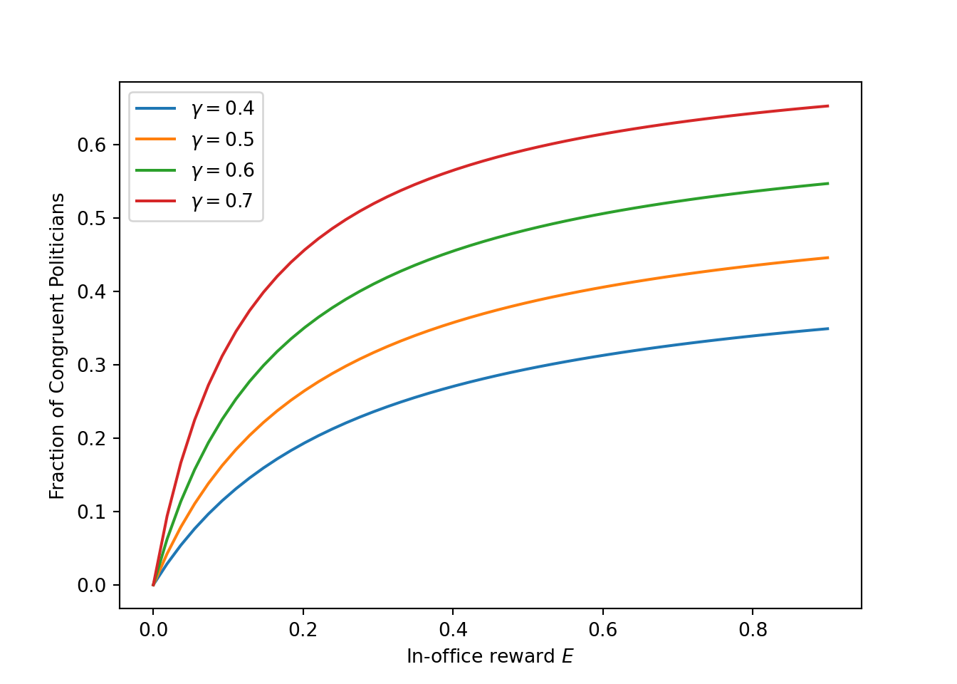
(Prediction 4) Paying higher wages will lead to the increase in the fraction of congruant politicians who will put themselves forward for office

Computational Implementation

I now implement the model in Python. I first start by importing several libraries.

import pandas as pd
import numpy as np
import scipy.stats
from matplotlib import pyplot as plt

import scipy.integrate
from scipy.optimize import fsolve

Then, I construct a class using several of the equations above:

class BesleyModel:
    
    def __init__(self, beta = 0.8, pi = 0.5, delta = 0.7, r_min = 0, E = 0.2, q = 0.2, R_max = 1):
        self.beta, self.pi = beta, pi
        self.delta, self.r_min, self.R_max = delta, r_min, R_max
        self.E, self.q = E, q
          
    def G(self, x):
        R_max, r_min = self.R_max, self.r_min
        
        return scipy.stats.uniform.cdf(x, loc = r_min, scale = R_max)
        
    def g(self, x):
        R_max, r_min = self.R_max, self.r_min
        
        return scipy.stats.uniform.pdf(x, loc = r_min, scale = R_max)
        
    def lbda(self, E):
        """
        Probability that dissonant politician does what the electorate wants
        """
        G = self.G
        q, beta = self.q, self.beta
        mu = (self.R_max - self.r_min)/2
        
        return q*G(beta*(mu+E))
    
    def phi(self, E):
        """
        Probability that firm term incumbent generates the good action for voters
        """
        pi = self.pi
        lbda = self.lbda
        
        return pi + (1-pi)*lbda(E)
    
    def Pi(self, E):
        """
        Updated probability that incumbent in congruent instead of dissonant
        conditional on generating a delta benefit in the first period
        """
        phi = self.phi
        pi = self.pi
        
        return pi/phi(E)
    
    def v(self, E):
        """
        Voter welfare viewed from the first period
        """
        delta, beta, pi = self.delta, self.beta, self.pi
        phi = self.phi
        
        return delta/(1-beta) * (phi(E) + pi*beta)/(1+beta*phi(E))
        

Then, I verify the predictions:

possible_E = np.linspace(0, 0.9, num=100)

#matrix for different pi's, beta's, whatever
possible_pi = [0.4, 0.5, 0.6, 0.7]

prob_congruence = np.empty([len(possible_E), len(possible_pi)])


def compute_prob(possible_E, possible_pi):
    
    for num, pi in enumerate(possible_pi):
        
        for num2, e in enumerate(possible_E):
            
            model=BesleyModel(beta = 0.7, pi = pi)
            prob_congruence[num2, num] = model.phi(E=e)
            
compute_prob(possible_E, possible_pi)

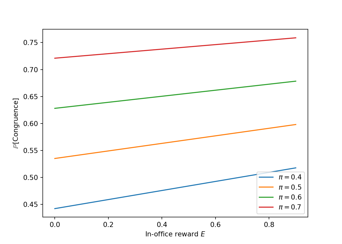
(Prediction 1) An increase in wages increases the probability of congruence between voter preferences and policy outcomes. As a consequence, it reduces turnover among first-term incumbents.

fig, ax = plt.subplots()

for i in range(prob_congruence.shape[1]):
    ax.plot(possible_E, prob_congruence[:,i], label = f'$\pi=${possible_pi[i]}')

    
ax.set_xlabel("In-office reward $E$")
ax.set_ylabel("$\mathbb{P}$[Congruence]")
ax.legend()

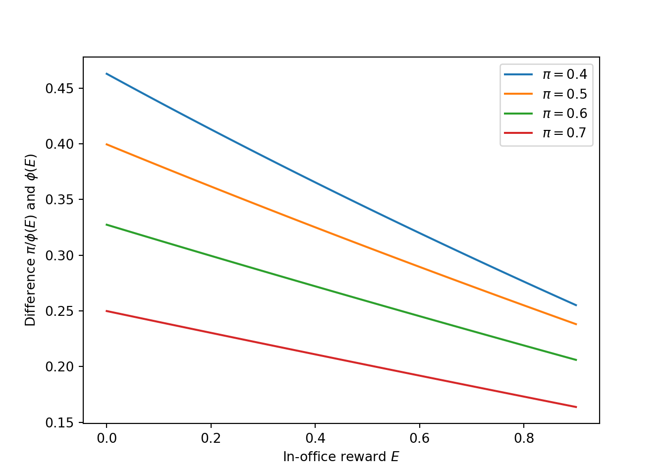
(Prediction 2) Conditional on electing a dissonant politician, behavior deteriorates over time. But politicians in their second term in office behave better on average than those in their first term. The difference between second-term and first-term incumbents is smaller the larger the politician’s wage.

possible_E = np.linspace(0, 0.9, num=100)

#matrix for different pi's, beta's, whatever
possible_pi = [0.4, 0.5, 0.6, 0.7]

prob_congruence = np.empty([len(possible_E), len(possible_pi)])


def compute_prob(possible_E, possible_pi):
    
    for num, pi in enumerate(possible_pi):
        
        for num2, e in enumerate(possible_E):
            
            model=BesleyModel(beta = 0.7, pi = pi)
            prob_congruence[num2, num] = (model.pi/model.phi(E=e) - model.phi(E=e))
            
compute_prob(possible_E, possible_pi)

fig, ax = plt.subplots()

for i in range(prob_congruence.shape[1]):
    ax.plot(possible_E, prob_congruence[:,i], label = f'$\pi=${possible_pi[i]}')

    
ax.set_xlabel("In-office reward $E$")
ax.set_ylabel("Difference $\pi/\phi(E)$ and $\phi (E)$")
ax.legend()

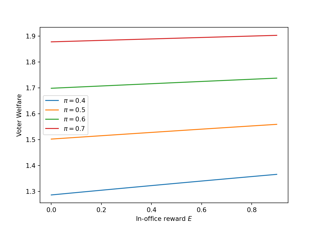
(Prediction 3) Increasing \(E\) increases voter welfare.

possible_E = np.linspace(0, 0.9, num=100)

#matrix for different pi's, beta's, whatever
possible_pi = [0.4, 0.5, 0.6, 0.7]

prob_congruence = np.empty([len(possible_E), len(possible_pi)])


def compute_prob(possible_E, possible_pi):
    
    for num, pi in enumerate(possible_pi):
        
        for num2, e in enumerate(possible_E):
            
            model=BesleyModel(beta = 0.7, pi = pi)
            prob_congruence[num2, num] = model.v(e)
            
compute_prob(possible_E, possible_pi)

fig, ax = plt.subplots()

for i in range(prob_congruence.shape[1]):
    ax.plot(possible_E, prob_congruence[:,i], label = f'$\pi=${possible_pi[i]}')

    
ax.set_xlabel("In-office reward $E$")
ax.set_ylabel("Voter Welfare")
ax.legend()

Endogenous Selection

Finally, I verify proposition 4, using a new class for the model with endogenous selection:

class BesleyModelEndogSel:
    
    def __init__(self, 
                 beta = 0.8, 
                 gamma = 0.5, 
                 E = 0.2, 
                 r_min = 0, R_max = 1,
                 w_max_c = 0.8, w_max_d = 1):
        
        self.beta, self.gamma = beta, gamma
        self.r_min, self.R_max = r_min, R_max
        self.mu = (self.R_max - self.r_min)/2
        self.E = E
        self.w_max_c, self.w_max_d = w_max_c, w_max_d
    
    def G(self, x):
        R_max, r_min = self.R_max, self.r_min
        
        return scipy.stats.uniform.cdf(x, loc = r_min, scale = R_max)
        
    def g(self, x):
        R_max, r_min = self.R_max, self.r_min
        
        return scipy.stats.uniform.pdf(x, loc = r_min, scale = R_max)
        
    def Lbda(self, E, w_bar):
        """
        Probability of congruent behavior by a randomly selected dissonant politician
        (the fraction of dissonant politicians willing to serve)
        """
        G = self.G
        beta = self.beta
        mu = (self.R_max - self.r_min)/2
        
        def integrand(w):
            
            G = self.G
            beta = self.beta
            mu = (self.R_max - self.r_min)/2
            return G(beta*(E+mu) - w)
        
        value = scipy.integrate.quad(integrand, 0, w_bar)[0]
        out = value / w_bar
        
        return out
    
    def Psi(self, x):
        """
        Helper function to solve functional equation
        """
        G, g = self.G, self.g
        beta = self.beta
        
        def integrand(y, x):
            
            G = self.G
            beta = self.beta
            mu = (self.R_max - self.r_min)/2
            
            return y*g(y)/(1+G(beta*x)*beta)
        
        out = - scipy.integrate.quad(integrand, 0, beta*x, args = (x,))[0]
        
        return out
    
    def solve_wbar(self):
        """
        Solve for the reservation wage among dissonant politicians
        """
        Psi = self.Psi
        E = self.E
        mu = self.mu
        
        def tosolve(w_bar, Psi, E, mu):
            
            return w_bar - E - mu - Psi(E + mu - w_bar)
        
        out = fsolve(tosolve, 1e-5, args=(Psi, E, mu))
        
        return out[0]
    
    def share_dissonant(self):
        """
        The share of dissonant politicians who are willing to become politicians
        """
        
        solve_wbar = self.solve_wbar
        w_max_d = self.w_max_d
        
        return(solve_wbar()/w_max_d)
    
    def pi(self):
        """
        Compute the share of consonant politicians in the pool of people willing to become politicians
        """
        E = self.E
        gamma = self.gamma
        solve_wbar = self.solve_wbar
        w_max_c, w_max_d = self.w_max_c, self.w_max_d
        
        w_bar = solve_wbar()
        
        return gamma*(E/w_max_c)/(gamma*(E/w_max_c) + (1-gamma)*(w_bar/w_max_d))
        
        
        

(Prediction 4) Paying higher wages will lead to the increase in the fraction of congruant politicians who will put themselves forward for office

possible_E = np.linspace(0, 0.9, num=50)

#matrix for different pi's, beta's, whatever
possible_gamma = [0.4, 0.5, 0.6, 0.7]

prob_congruence = np.empty([len(possible_E), len(possible_gamma)])


def compute_prob(possible_E, possible_gamma):
    
    for num, gamma in enumerate(possible_gamma):
        
        for num2, e in enumerate(possible_E):
            
            model=BesleyModelEndogSel(beta = 0.7, E = e, gamma = gamma)
            prob_congruence[num2, num] = model.pi()
            
compute_prob(possible_E, possible_gamma)

fig, ax = plt.subplots()

for i in range(prob_congruence.shape[1]):
    ax.plot(possible_E, prob_congruence[:,i], label = f'$\gamma=${possible_gamma[i]}')

    
ax.set_xlabel("In-office reward $E$")
ax.set_ylabel("Fraction of Congruent Politicians")
ax.legend()

Conclusion

All the propositions are verified graphically in the blog post. This illustrates the dynamics in the Besley model. I hope I have done a good job distinguishing the three mechanisms, and I hope I have provided a tangible computational implementation of the model. Thank you for reading!