Spatial Operations in R

Introduction

In this post, I will demonstrate some useful spatial operations in R. In particular, I want to do some spatial data wrangling to generate a border between two areas on a particular map, and afterwards, compute the distance of each polygon (area) to that border. This is something that is often featured in spatial regression discontinuity designs, where the “running” variable is the distance (positive or negative) from the border, the border being, for example, ancient borders, an area of exploitation, some territory impacted by some event, or some seized territory.

I will confine myself to these things in this post:

• Combining a map of the Roman Empire (around 200AD) with a contemporary map of Dutch municipalities, thereby tracking which contemporary municipalities fell within the border of the Roman Empire about 2000 years ago.
• Extracting a border
• Making the border potentially more precise and reliable.
• Calculating the distance to the border

In another blog post, I’ll also detail how to digitize and customize historical maps, as I found the available online resources to be insufficiently clear. One good reference article for this type of task is Giuliano and Matranga (2020), but even that is far from a self-contained guide, and is focused on ArcGIS, a paid piece of software.

To start off, we load the libraries we need during this session:

library(tidyverse)
library(rgeos)
library(sf)
library(spatialrisk)

Merging a map

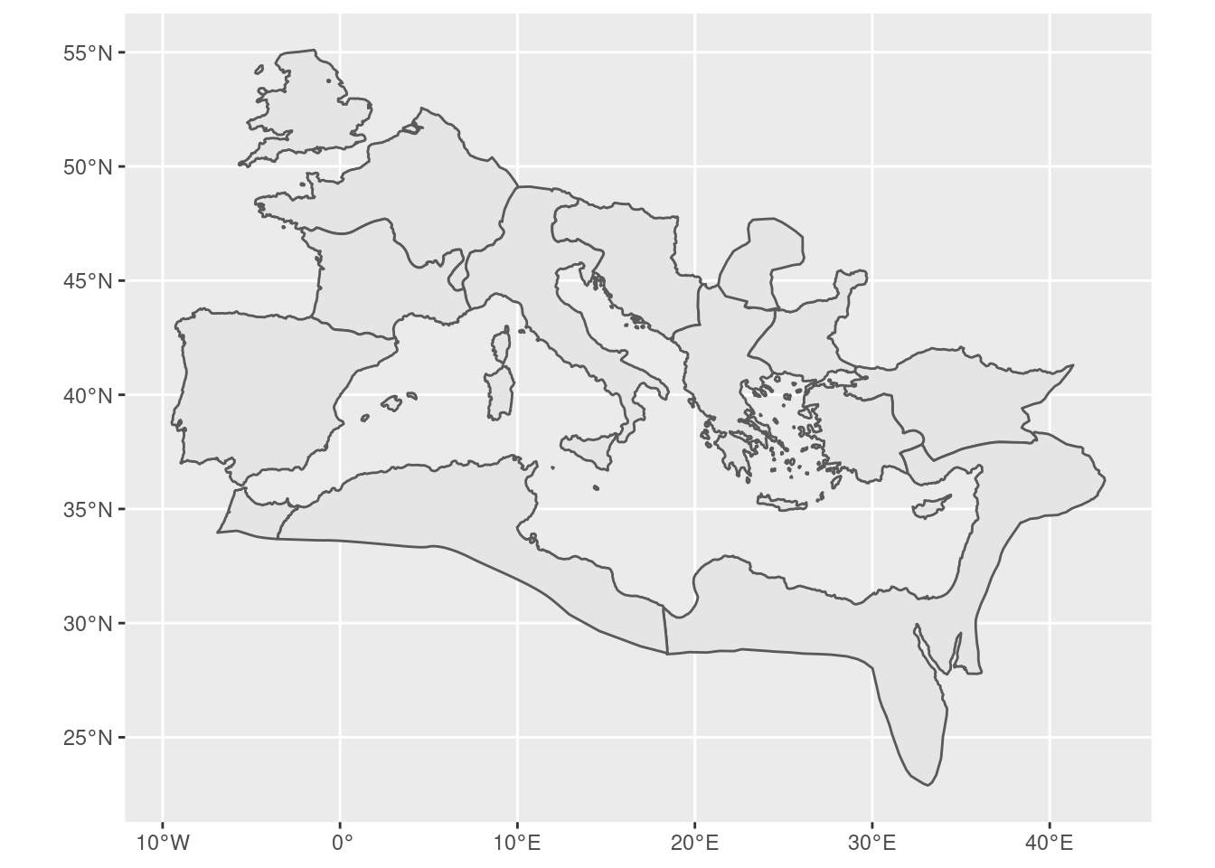
First, we load in the map of the Roman Empire. The cawd package, courtesy of the Ancient World Mappign Center, features several maps of the ancient world, among which is the Roman Empire and its borders in several years. It provides the maps in SpatialPolygons objects, whereas we are going to work with the sf package and spatialFeatures. Hence we first transform it:

rom <- cawd::awmc.roman.empire.200.sp
rom <- sf::st_as_sf(rom)

The map looks as follows:

rom |> 
  ggplot() + geom_sf()

We can find out what projection is used:

sf::st_crs(rom)$input

## [1] "+proj=longlat +datum=WGS84 +ellps=WGS84 +towgs84=0,0,0"

.. which is a standard WGS84 projection. For our purposes, it is important that the maps use the same projection, otherwise it is not possible to do operations on them jointly.

Changing a projection is possible by, for example:

st_transform(rom, 32119) |>
  ggplot() + geom_sf()

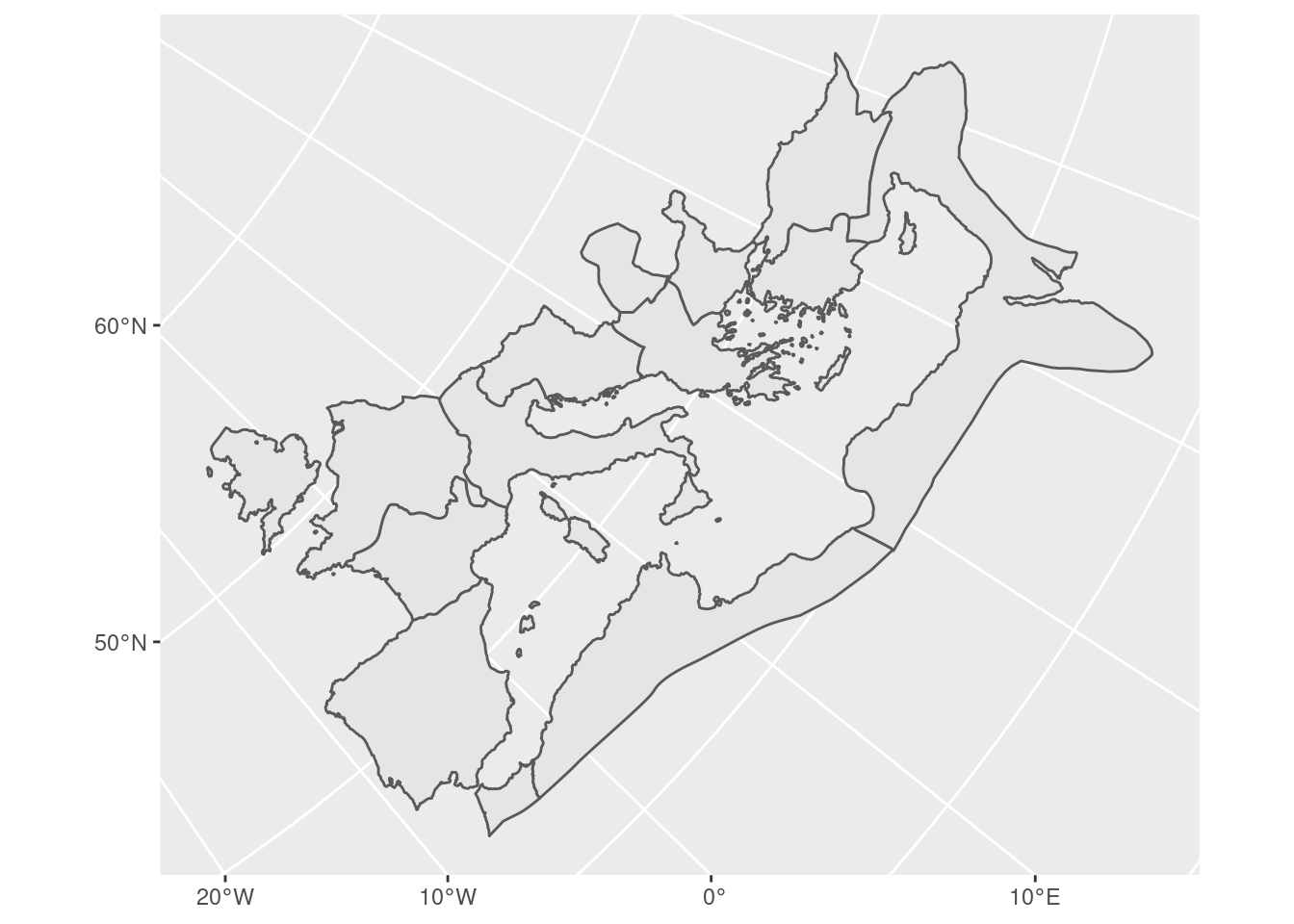
You can find interesting projections on, for example https://epsg.io/map, searching and leaving the search bar empty. This will give you a list of possible projection. You can of course also search. Two similar websites are SpatialReference.org and PROJ.org.

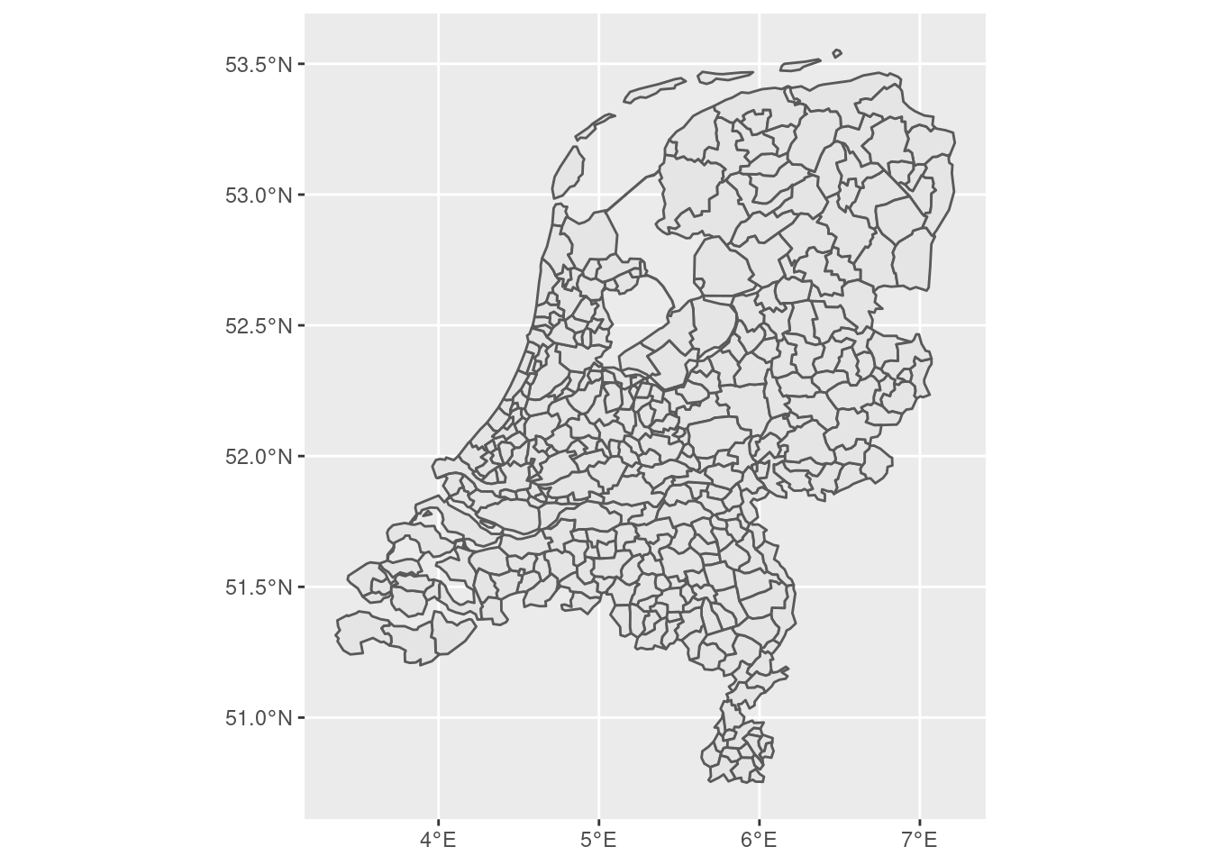
Now, let’s load in a map containing municipalities. For brevity, I’ll use the 2018 Dutch municipalities from the spatialrisk package.

gem <- spatialrisk::nl_gemeente
sf::sf_use_s2(FALSE)

gem |> ggplot() + geom_sf()

Then, I use the st_contains function to find out which of the municipalities are contained in the Roman Empire. st_contains tests whether each geometry in a set of query geometries is contained within any of a set of target geometries.

The difference between st_contains() and st_within() is that st_contains() checks whether one geometry is completely contained within another, while st_within() checks whether one geometry is completely within the interior of another (i.e., inside the other geometry, with no points on the boundary).

The st_contains() function is one of several functions in sf that can be used to test spatial relationships between geometries. Other similar functions include:

• st_intersects(): Tests whether two sets of geometries intersect.
• st_touches(): Tests whether two sets of geometries touch at any point, but do not intersect.
• st_within(): Tests whether each geometry in a set is within another set of geometries.
• st_overlaps(): Tests whether two sets of geometries overlap each other.

st_intersects checks whether there is any intersection at all, so that is the least strict function.

overlap <- st_contains(rom, gem)

The output of st_overlaps, saved in overlap, contains 112 elements. For each of the 112 polygons in rom, it tells us with which of the 352 partially or entirely overlap with one of the geometries in rom. Let us now extract all of those numbers:

numbers <- map(overlap, function(x) {x}) |> reduce(c)

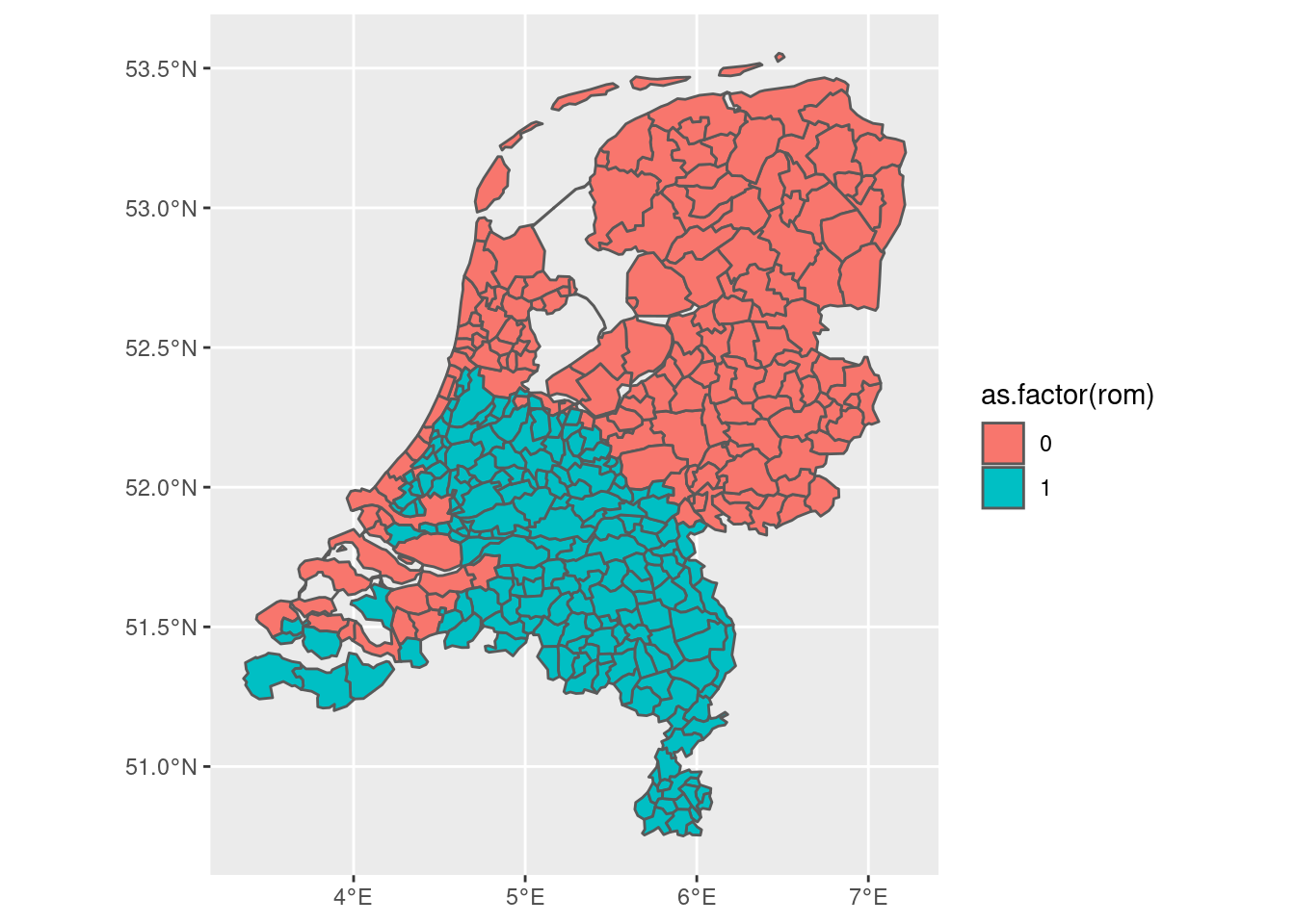
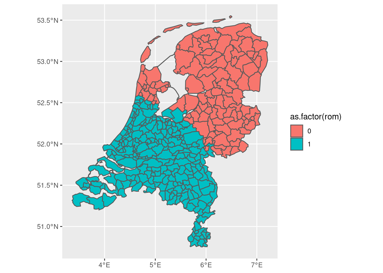
From which we find that 189 municipalities overlap with the former Roman Empire. To find out which ones, we can integrate that into the gem data.frame as follows:

gem2 <- gem |>
  mutate(rom = if_else(is.element(id, numbers), 1, 0))

gem2 |> ggplot(aes(fill = as.factor(rom))) + geom_sf()

We can also do this in a slightly different way. A disadvantage of the preceding approach is that we might also include municipalities with only a 10% overlap, whereas we want to include only municipalities that have a substantial, say, 50% overlap. We might want to compute the intersection between the two data.frames and then calculate the area of overlap:

crude <- st_intersects(rom, gem)
crude_nos <- map(crude, function(x) {x}) |> reduce(c)

gem3 <- gem |>
  mutate(rom = if_else(is.element(id, crude_nos), 1, 0))

gem3 |> ggplot(aes(fill = as.factor(rom))) + geom_sf()

Finally, maybe the one is a little bit too conservative whereas the other is a little bit too crude. We might want to decide explicitly based on the area of overlap. The way in which we could do that is as follows:

# Make the intersection and cutoff the data.frame at the borders
intersect <- st_intersection(rom, gem)
intersect <- intersect |> select(id, code, areaname, geometry)

# Calculate the areas of all municipalities in the gem data.frame
gem_ar <- gem |> 
  select(id, code, areaname, geometry) |> 
  rename(geometry_large = geometry) |>
  mutate(area_large = st_area(geometry_large))

gem_ar |> head(5)

## Simple feature collection with 5 features and 4 fields
## Geometry type: MULTIPOLYGON
## Dimension:     XY
## Bounding box:  xmin: 5.124677 ymin: 52.25261 xmax: 7.100014 ymax: 53.31012
## Geodetic CRS:  WGS 84
##   id   code    areaname                 geometry_large      area_large
## 1  1 GM0014   Groningen MULTIPOLYGON (((6.772527 53... 193756466 [m^2]
## 2  2 GM0034      Almere MULTIPOLYGON (((5.350772 52... 141345387 [m^2]
## 3  3 GM0037 Stadskanaal MULTIPOLYGON (((7.015446 53... 121754152 [m^2]
## 4  4 GM0047     Veendam MULTIPOLYGON (((6.961735 53...  78299593 [m^2]
## 5  5 GM0050    Zeewolde MULTIPOLYGON (((5.58907 52.... 253523368 [m^2]

# Calculate the areas of all municipalities in the intersected data.frame
intersect <- intersect |>
  mutate(area_small = st_area(geometry)) |>
  st_drop_geometry()

intersect |> head(5)

##     id   code  areaname      area_small
## 6    2 GM0034    Almere   2418600 [m^2]
## 6.1  5 GM0050  Zeewolde   1986671 [m^2]
## 6.2 45 GM0202    Arnhem  33664091 [m^2]
## 6.3 46 GM0203 Barneveld 103850548 [m^2]
## 6.4 47 GM0209 Beuningen  47523926 [m^2]

# Filter the observations based on the ratio between the areas
# in the intersect and gem data.frames
final <- gem_ar |> left_join(intersect) |>
  mutate(ratio = area_small / area_large)

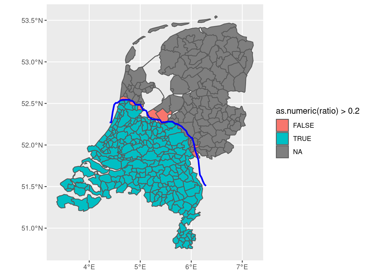
Then we could plot which municipalities we include based on a certain threshold, e.g. 20%:

final <- final |>
  mutate(include = if_else(as.numeric(ratio) > 0.2, 1, 0)) 

final |>
  ggplot(aes(fill = include)) + geom_sf()

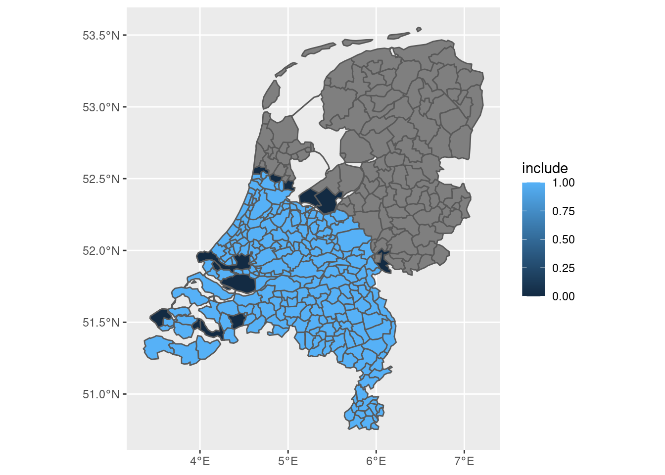
This seems near-perfect, as we can now:

• Distinguish between “fuzzy” and “absolute” municipalities.
• Control the threshold ourselves
• Decide which municipalities to include based on this threshold
• Consider that some municipalities didn’t actually exist in 200AD because of the creation of new land (those are some of the dark blue areas!)

Extracting a border

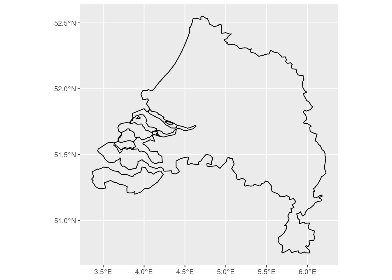
Now, let’s use final with the condition that ratio > 0.2 and find the border:

boundary <- st_union(final |> filter(as.numeric(ratio) > 0.2)) |> st_boundary()

We did this by first merging all polygons of municipalities together based on the condition that ratio be greater than 0.2, and then extracting the outer boundary of that polygon:

boundary |> ggplot() + geom_sf()

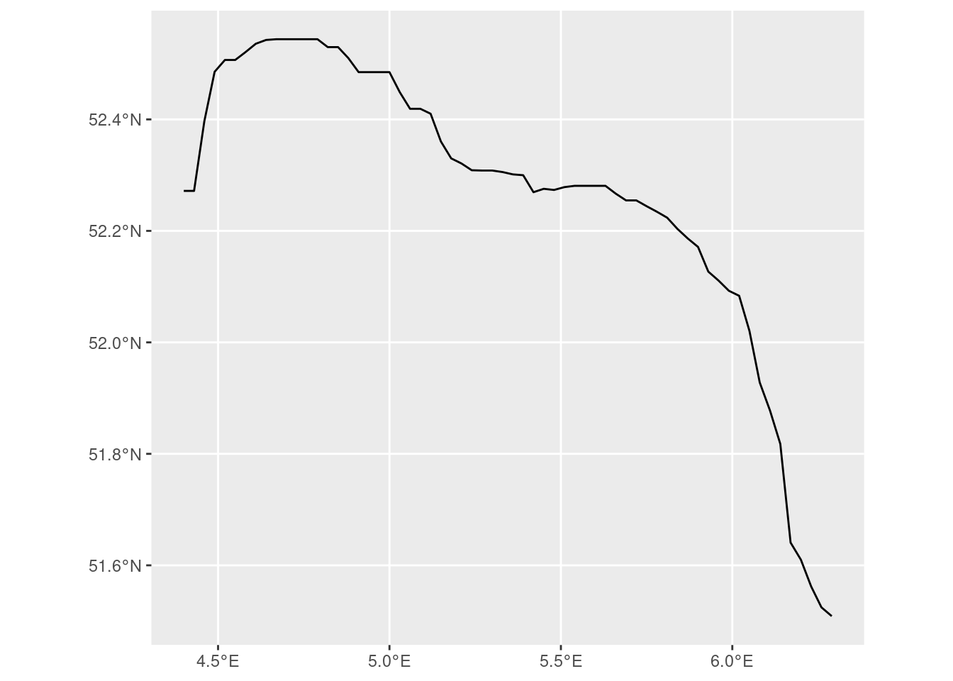
One way now to find the distance to the border is to naively use the entire border:

final_dist <- final %>%
  mutate(distance = as.numeric(st_distance(boundary, final)))

final_dist |> ggplot(aes(fill = distance < 10000)) + geom_sf()

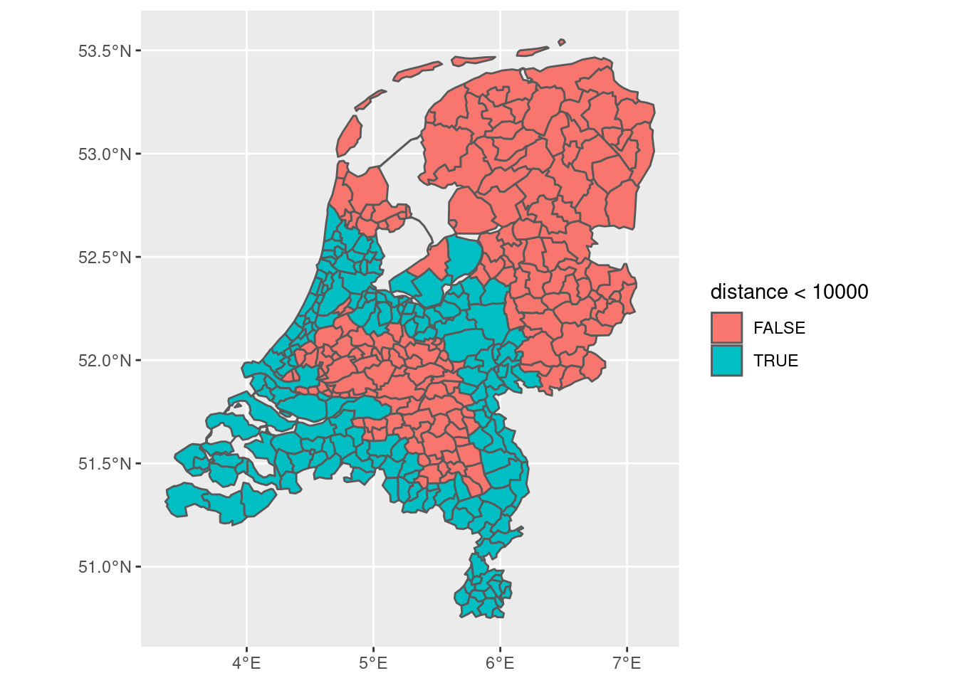
Of course, we only want to consider the distance from the northern border, as the other borders are not actually borders of the former Roman empire. We therefore have to make the border a little bit more precise.

Making the border more precise (I)

We can do this by only considering the northern part of the border and by iterating through the latitudes from a start to an end point. Then, we can extract only the relevant part of the border based on an interpolation:

• First, we extract the boundary and group and find the northern-most coordinate:

spl <- boundary %>% 
  st_cast("POINT") %>% 
  as("Spatial")

spl_grouped <- spl@coords %>% 
  as.data.frame() %>%
  group_by(coords.x1) %>% 
  arrange(coords.x1) %>% 
  slice_max(coords.x2)

spl_grouped

## # A tibble: 557 × 2
## # Groups:   coords.x1 [546]
##    coords.x1 coords.x2
##        <dbl>     <dbl>
##  1      3.36      51.3
##  2      3.37      51.4
##  3      3.37      51.3
##  4      3.37      51.3
##  5      3.38      51.3
##  6      3.39      51.3
##  7      3.41      51.3
##  8      3.43      51.4
##  9      3.43      51.5
## 10      3.44      51.4
## # … with 547 more rows

• Secondly, we can start from a given latitude, and find the maximum longitude for that point to only extract the northern border. I introduce two parameters, the one for interpolating between the param highest points, and the other param2 for the granularity of selecting points throughout the loop.

latitudes <- seq(4.4, 6.3, by = 0.03)
param <- 3
param2 <- 0.1

interpolation <- latitudes %>%
  map_dbl(function(x) { 
    spl_grouped %>%
      ungroup() %>%
      filter(between(coords.x1, x - param2, x + param2)) %>%
      slice_max(coords.x2, n = param) %>%
      pull(coords.x2) %>% 
      mean()
    })

line <- st_linestring(matrix(c(latitudes, interpolation), ncol = 2))
line_sfc <- st_sfc(line, crs = st_crs(4326))
line_sf <- st_sf(geometry = line_sfc)

line_sf |> ggplot() + geom_sf()

Now, we can integrate this new line into our original gem2 data.frame and calculate the distance to it:

df <- line_sf %>%
  rename(geometry_large = geometry) |>
  mutate(id = 1000, code = NA, areaname = 'border', area_large = NA, area_small = NA) %>%
  bind_rows(final)

ggplot() +
  geom_sf(data = df %>% filter(areaname != 'border'), aes(fill = as.numeric(ratio) > 0.2)) +
  geom_sf(data = df %>% filter(areaname == 'border'), color = 'blue', size = 1)

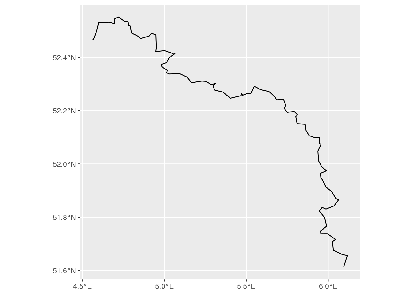
Making the border more precise (II)

We can also make the border more precise in a different way. We can just manually define a polygon that encapsulates the border in a nice and specific way. Then, we capture the border in this polygon, and then ask sf to return us the intersection of the polygon and the relevant piece of the border. I think this is generally the nicest way.

point1 <- c(4.5, 52.5)
point2 <- c(4.5, 53)
point3 <- c(6.3, 53)
point4 <- c(6.3, 51.5)
point5 <- c(4.5, 52.5)

coords <- list(rbind(point1, point2, point3, point4, point5))
poly_coords <- st_polygon(coords)

poly_c <- st_sfc(poly_coords, crs = st_crs(4326))
poly_l <- st_sf(poly_c) |> rename(geometry = poly_c)

boundary <- st_sf(boundary) |> rename(geometry = boundary)

new_boundary <- st_intersection(boundary, poly_l)

new_boundary |> ggplot() + geom_sf()

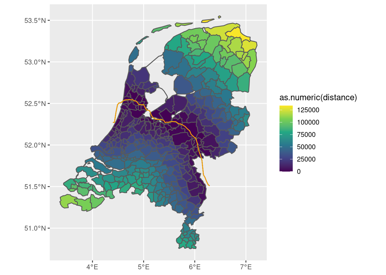
Calculating the distance

Calculating the distance can then be done as follows. With the first border:

df <- df |>
  mutate(distance = st_distance(df, line_sf))

df |> ggplot(aes(fill = as.numeric(distance))) + 
  geom_sf() + 
  geom_sf(data = df |> filter(areaname == 'border'), color = 'orange') +
  scale_fill_continuous(type='viridis')

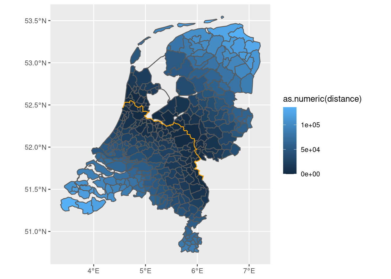
And with the second border:

final |> 
  mutate(distance = st_distance(final, new_boundary)) |>
  ggplot() + geom_sf(aes(fill = as.numeric(distance))) +
  geom_sf(data = new_boundary, color = 'orange')

This object can then be used to determine the distance from the border, as a cut-off point or as auxiliary variable to the cut-off point.

• For example, you can take the municipalities that are closest to the border, but inside the Roman empire, and use that to define the distance of all other municipalities to one of their centroids. That could then be used as a running variable.
• You could also just naively use the border as the running variable.
• Or you could fine-tune the interpolation so that the border overlaps precisely with the municipal boundaries.

Conclusion

Hopefully, I have demonstrated how to create variables that map to the distance to a certain border, used in spatial regression discontinuity designs. If you have any questions, feel free to contact me. Thanks for reading!