How to create a running variable in a spatial RDD?

By Bas Machielsen

May 14, 2024

Introduction

In this post, I’ll explain, using R code, how to create a distance to the border and an associated running variable often met in geographic regression discontinuity designs. Depending on your data, this can be kind of difficult, so I’ll explain this using two examples:

One using raster data, computing distance to the border of the Roman Empire, inspired by a teaching project
One using vector data, computing distance to the Veneto-Lombardo border, inspired by a research project with Giacomo Domini.

The difference between these examples is that, in the first case, I have a geographic variable allowing me to easily determine on which side of the border you are. In the second case, I have not, so I need to resort to a slightly more refined method.

Also, I think it is illustrative to show examples using both raster and vector data.

Case I: Roman Empire

For this, I’m using the border of the Roman Empire and combine this with a dataset of countries now encompassing the Roman border. I need these libraries:

library(cawd)
library(rnaturalearthdata)
library(tidyverse)
library(sf)
library(stars)
library(starsExtra)

I now download the maps of Europe and of the Roman Empire:

europe <- rnaturalearthdata::sovereignty50 |>
  st_as_sf() |>
  filter(continent == "Europe")

re <- cawd::awmc.roman.empire.117.sp |> st_as_sf()

I extract the border of the Roman Empire and focus on the northern border:

boundary_re <- st_boundary(re)

# Extract Northern Border Roman Empire
countries_with_north_border <- europe |> filter(is.element(sovereignt, c("Netherlands", "Germany", "Croatia",
                                                                   "Austria", "Hungary", "Slovakia",
                                                                   "Ukraine", "Romania", "Bulgaria",
                                                                   "Republic of Serbia")))

# Filter the LINESTRING(s) with the maximum Y-coordinate
northernmost_lines <- st_intersection(boundary_re, countries_with_north_border)

Finally, I have to delete a small part of the non-northern border in Croatia:

# Filter out south border of Croatia
coords <- matrix(c(
  15, 46,
  20, 42,
  10, 42,
  10, 46,
  15, 46), ncol = 2, byrow = TRUE)

# Create a polygon object
polygon <- st_polygon(list(coords)) |>
  st_sfc(crs = 4326)

northernmost_border <- northernmost_lines |> 
  st_difference(polygon)

Since I am planning to use a raster dataset, I will now create a buffer around the border, and on the basis of that, create a raster grid:

# Build Buffer Around Roman Empire Border and Intersection With Europe
sf_use_s2(TRUE)
buffer_around_northern_border <- st_buffer(northernmost_border, 200000)

# Intersection with Europe
sf_use_s2(FALSE)
area_around_re_border <- europe |>
  st_intersection(buffer_around_northern_border)

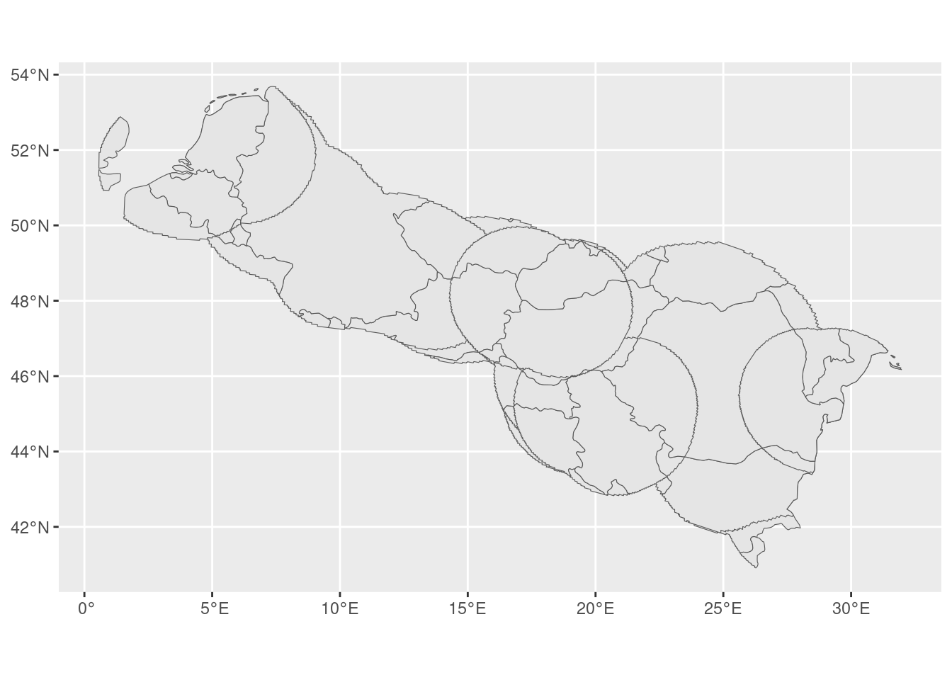
# Check what this area looks like
area_around_re_border |>
  ggplot() + geom_sf()

Now, I am creating an sf grid, and then convert it to raster using the stars and starsExtra packages:

# Build a grid on this basis
grid <- st_make_grid(area_around_re_border,  n = 100) 
filter <- st_within(grid, st_union(area_around_re_border)) |> lengths() > 0

# Check grid
final_grid <- grid[filter]

# Turn grid into an empty raster and save
raster_grid <- grid[filter] |> stars::st_as_stars() 
final_raster_grid <- raster_grid[raster_grid['values'] ==1]

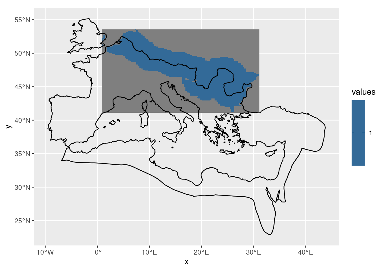
This looks as follows:

ggplot() + 
  geom_stars(data=final_raster_grid) +
  geom_sf(data=boundary_re)

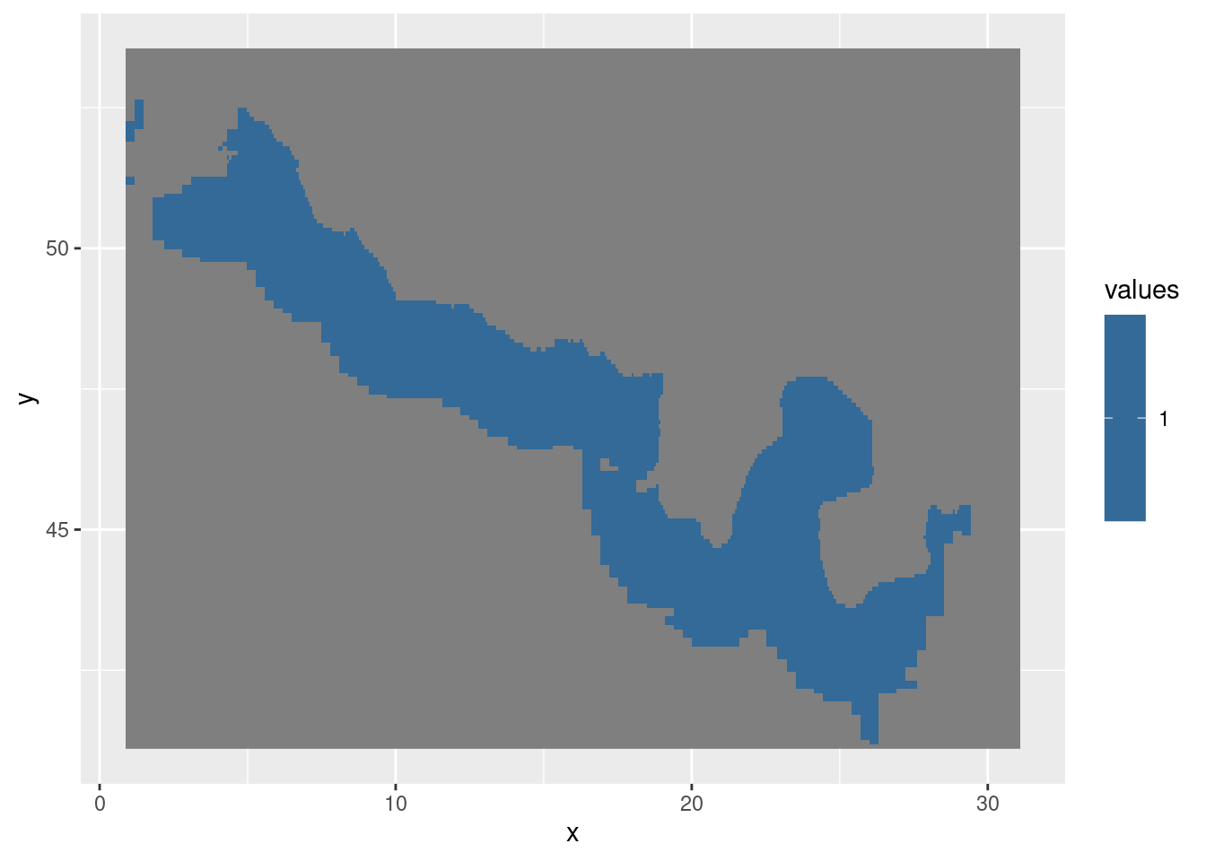
And it can even be masked by an sf object, something we’ll make use of:

ggplot() + geom_stars(data=final_raster_grid[re])

Finally, we’ll create a distance to the border variable using the dist_to_nearest function and write it as an attribute in the raster:

# Create distance to the border:
nearest_feat <- starsExtra::dist_to_nearest(final_raster_grid, northernmost_lines)
final_raster_grid$distance <- nearest_feat$d

To create a distance variable, we now create a variable indicating whether a grid cell is inside the Roman Empire:

# Create indicator for being inside RE
grid_sf <- st_as_sfc(final_raster_grid, as_points=T)  
logical <- as.logical(st_within(grid_sf, re))
final_raster_grid <- final_raster_grid |>
  mutate(inside_re = case_when(!is.na(logical) & values == 1 ~ 1, 
                               is.na(logical) & values == 1 ~  0,
                               TRUE ~ NA))

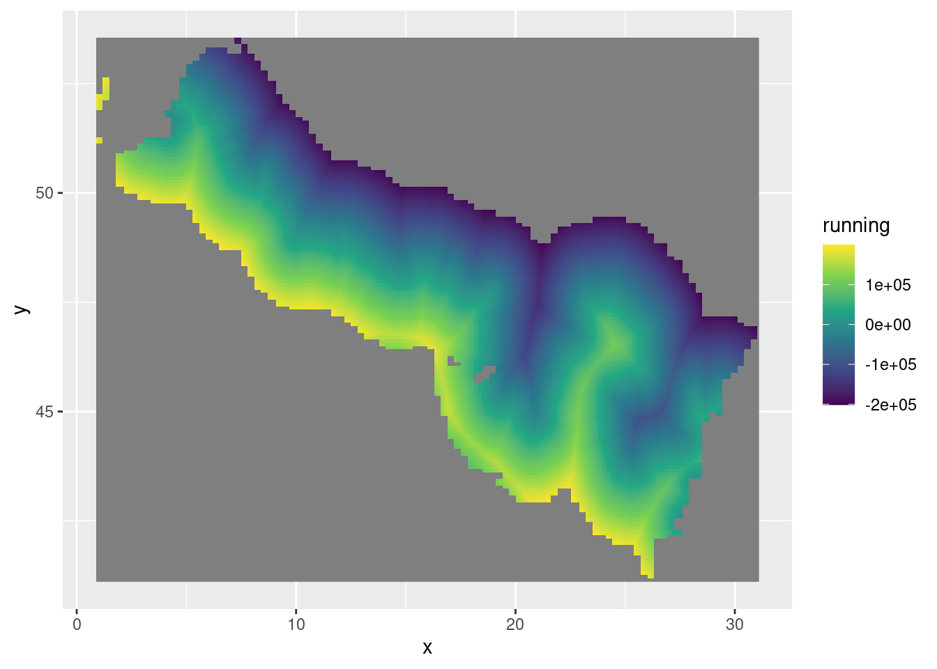
Then, the running variable is just defined as distance if the grid cell is inside the Roman Empire, and -distance otherwise:

# Create the running variable
final_raster_grid <- final_raster_grid |> 
  mutate(running = if_else(inside_re == 1, distance, -distance))

This looks as follows:

ggplot() + 
  geom_stars(data=final_raster_grid['running']) + 
  scale_fill_viridis_c()

Case II: Veneto-Lombardo

In this case, we don’t have an object like re telling us on which side of the border a particular polygon is. First, we import the border and load the shapefile of municipalities:

# Import the border
border <- st_read('./shapefile/shapefile_italy_1860.shp') |>
  dplyr::filter(id == 5)

## Reading layer `shapefile_italy_1860' from data source 
##   `/home/baswork/Documents/git/new_website/content/blog/2024-05-14-how-to-create-a-running-variable-in-a-spatial-rdd/shapefile/shapefile_italy_1860.shp' 
##   using driver `ESRI Shapefile'
## Simple feature collection with 5 features and 2 fields
## Geometry type: MULTILINESTRING
## Dimension:     XY
## Bounding box:  xmin: 9.61294e-05 ymin: 0.0004079144 xmax: 13.90954 ymax: 47.09096
## Geodetic CRS:  WGS 84

# Load the municipalities
italy_municipalities <- giscoR::gisco_get_lau(country='Italy', year='2016')

# Load the provinces - to filter the relevant municipalities
italy_provinces <- giscoR::gisco_get_nuts(country='Italy', nuts_level='3', year='2016') |> 
  mutate(prov_code =  str_sub(NUTS_ID, 1, 4)) |> 
  filter(is.element(prov_code, c('ITC4', 'ITH3')))

# Filter the relevant municipalities
# Combine overlaps and within
filter_indication <- st_within(italy_municipalities, italy_provinces, sparse=TRUE) 
filter_indication2 <- st_overlaps(italy_municipalities, italy_provinces, sparse=TRUE) 
mask <- apply(filter_indication, 1, any)
mask2 <- apply(filter_indication2, 1, any)
final_mask <- map2_lgl(mask, mask2, ~ any(.x + .y))
relevant_part <- italy_municipalities[final_mask,]

The shapefile now looks like this:

# Plot to check
ggplot() + geom_sf(data=relevant_part) + geom_sf(data=border, color='blue')

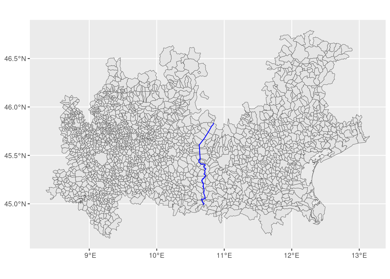
The problem is that the contemporary provinces don’t exactly match the old ones which we need, so we cannot rely on contemporary data. Instead, we have to find which side of the border each place is located by looking at the angle between the polygon centroid and the border.

# Spatial join
relevant_part <- st_join(relevant_part, italy_provinces, join=st_nearest_feature)
# Calculate centroids of polygons in relevant_part
relevant_centroids <- st_centroid(relevant_part)

# Calculate nearest point on the line for each centroid
nearest_points <- st_nearest_points(relevant_centroids, border)

# Calculate the angle between the line connecting centroids and their nearest points on the border
angles <- numeric(length(nearest_points))
for (i in seq_along(nearest_points)) {
  centroid_coords <- st_coordinates(relevant_centroids[i,])
  nearest_coords <- st_coordinates(nearest_points[i])

  # Calculate the X and Y differences (endpoint - origin)
  delta_y <- nearest_coords[2, 2] - nearest_coords[1, 2]
  delta_x <- nearest_coords[2, 1] - nearest_coords[1, 1]
  
  # Calculate the angle using atan2
  angle_radians <- atan2(delta_y, delta_x)
  angles[i] <- angle_radians * (180 / pi)
}

# Add angles to relevant_part
relevant_part$angle_to_line <- angles
relevant_part$group <- if_else(abs(relevant_part$angle_to_line) > 90, "Veneto", "Lombardia")

Then, after running this algorithm, we get the following:

relevant_part |> 
  ggplot(aes(fill=group)) + geom_sf()

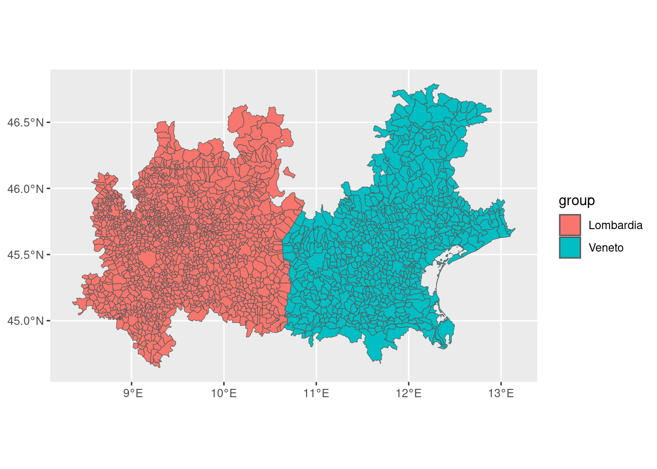
..which is what we set out to accomplish! Thanks for reading this post.

Posted on:: May 14, 2024

Length:: 5 minute read, 991 words

See Also: