Intervals and Durations in Feeding a New-born :)
By Bas Machielsen
June 2, 2024
Introduction
As those of you who might know me know, we (my wife and me) became parents a couple of months ago of a son named Lev. Apart from being a really cool guy, he’s also quite unpredictable in his tendencies for asking to be fed. We’ve been using an app called Huckleberry to record all feeding times and duration, and since he can be quite demanding, we were wondering about the relationship between feeding duration and times (intervals) between feeding.
As some of you might know, feeding a new-born can be quite demanding and this analysis might even be practical in the sense that, since there’s some agency the mother has over feeding her child, a mother might look for feeding policy that might decrease the burden a bit.
But who am I kidding, it’s just fun to analyze these very personal data. In the meantime, I’ll also take the time to discuss the quite new tinytable R package, a new table creating package that seems to be up and coming. Hopefully, after a couple of posts I’ll feel at home enough to begin writing my papers using it: it seems very user friendly.
Importing and Data Wrangling
To start out, I’ll load three package we’ll be needing and start importing my data file:
library(tidyverse)
library(modelsummary)
library(tinytable)
This is what the raw data look like:
lev <- read_delim('./c7d82626-bd81-4d48-a96f-09dc4209a560.csv')
## Rows: 1289 Columns: 8
## ── Column specification ────────────────────────────────────────────────────────
## Delimiter: ","
## chr  (6): Type, Duration, Start Condition, Start Location, End Condition, Notes
## dttm (2): Start, End
##
## ℹ Use `spec()` to retrieve the full column specification for this data.
## ℹ Specify the column types or set `show_col_types = FALSE` to quiet this message.
lev
## # A tibble: 1,289 × 8
##    Type  Start               End                 Duration `Start Condition`
##    <chr> <dttm>              <dttm>              <chr>    <chr>
##  1 Feed  2024-06-02 16:08:00 2024-06-02 16:29:00 00:20    00:10R
##  2 Feed  2024-06-02 12:45:00 2024-06-02 13:29:00 00:44    00:21R
##  3 Feed  2024-06-02 08:36:00 2024-06-02 09:22:00 00:46    00:46R
##  4 Feed  2024-06-02 06:00:00 2024-06-02 06:19:00 00:19    Null r
##  5 Feed  2024-06-02 01:09:00 2024-06-02 01:45:00 00:36    00:36R
##  6 Feed  2024-06-02 00:36:00 2024-06-02 00:47:00 00:11    Null r
##  7 Feed  2024-06-01 21:21:00 2024-06-01 21:31:00 00:09    00:09R
##  8 Feed  2024-06-01 20:28:00 2024-06-01 20:47:00 00:18    00:06R
##  9 Feed  2024-06-01 17:56:00 2024-06-01 18:31:00 00:34    00:17R
## 10 Feed  2024-06-01 14:37:00 2024-06-01 15:08:00 00:30    00:20R
## # ℹ 1,279 more rows
## # ℹ 3 more variables: `Start Location` <chr>, `End Condition` <chr>,
## #   Notes <chr>
I need to do a couple of things: I want to extract the month since I need to know how old our son was (he was born at the beginning of the month), and I want to calculate the interval from each feeding to the next. I do that before anything else since we’ve also bottle-fed him without time duration. We want those observations to be NA’ed rather than to be taken into account, since inclusion of those observations and disregarding bottle feedings might overestimate greatly the time between feeding.
Then, I calculate the interval between feeding, defined as the time between the Start of feeding at \(t\) and the End of the feeding at \(t-1\). There is a Duration variable there as well for the time a feeding takes, which I take to be an independent variable.
I also create a variable called day, which is a unique month-day indicator, since I want to estimate the relationship using within-day data (new-born children might have really “good” and “bad” days, so it might be useful to compare within-day and across-day estimates).
Finally, new-born children, at least after some time, start to acquire day and night rhythms, so we might include “night” as a possible control variable, since the default time between feedings is different at night than during the day. We define “night” to be any time between 9 o’clock in the evening (sadly, this is realistic) and 8 o’clock in the morning.
lev <- lev |>
  mutate(month = month(Start),
         interval = seconds(Start - lead(End)),
         Duration = parse_time(Duration),
         day = paste0(day(Start), "-", month(Start)),
         night = if_else(between(hour(Start), 0, 8) | between(hour(Start), 21, 23), 1, 0))

lev <- lev |>
  mutate(Duration = seconds(Duration))
After parsing all of this, I convert the Duration variable to seconds. Interval is also defined in seconds. This helps later to interpret our estimates.
Analysis: All Data
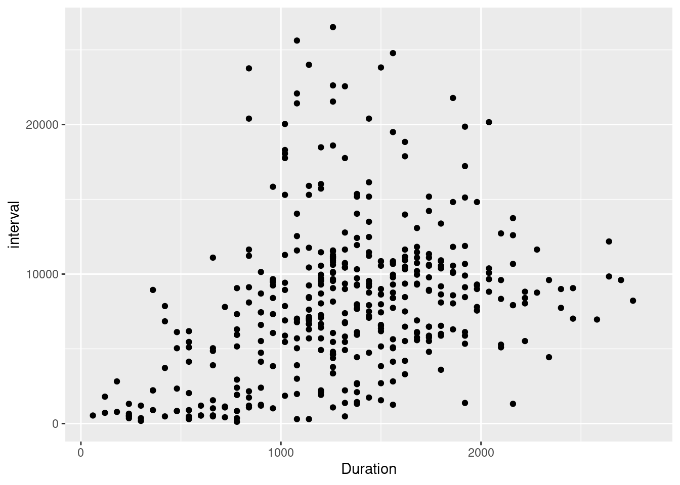
My first analysis focuses on all data I have since birth. Like I said, I want to exclude bottle feedings since I don’t have registered the time for them, and I throw out a couple of NA observations. Then, I visually inspect the relationship between Duration and interval between feedings.
filtered_lev <- lev |>
  filter(Type == "Feed", !is.na(End))

filtered_lev |>
  ggplot(aes(x=Duration, y = interval)) + geom_point()

library(fixest)
model_no_fe <- feols(fml = as.numeric(interval) ~ Duration + night, data = filtered_lev, vcov='hc1')
model_fe <- feols(fml = as.numeric(interval) ~ Duration + night | day, data = filtered_lev, vcov='hc1')
Considering this, we might think there’s a positive relationship between feeding time and interval between feedings, which we might have expected. The existence of this is some good news, as mothers can decide to feed longer (provided the baby wants to) to give themselves a longer break in between feedings as a matter of policy. Well, maybe.. I also estimate two regression models, which I report later.
Analysis: Data From 2 Months Onw
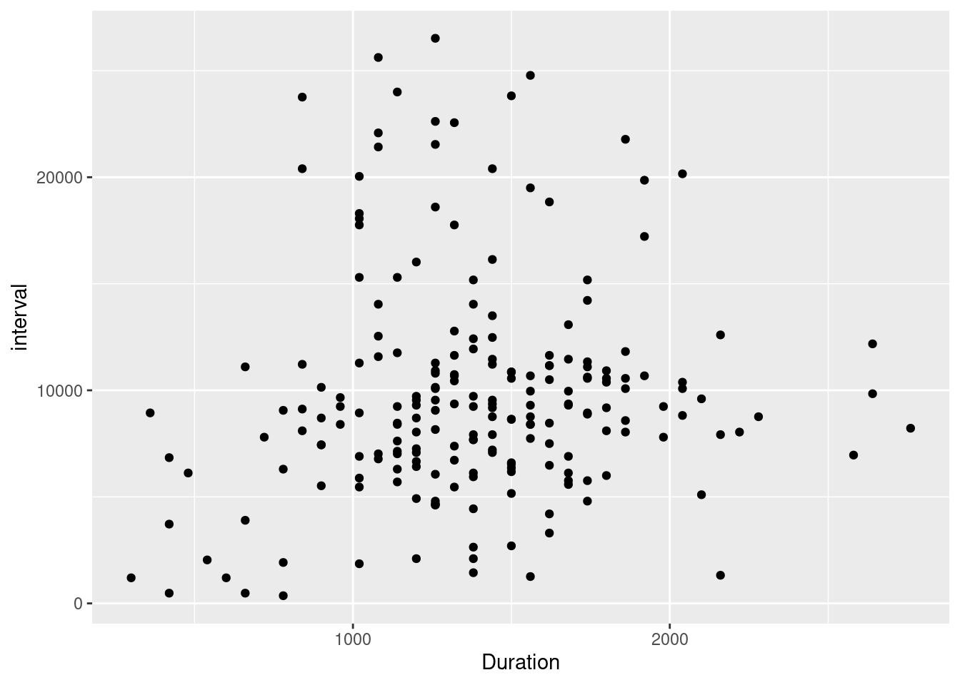
The next analysis repeats this, but uses data from 2 months after birth onward. The idea is that behavior should become a little more systematic after 2 months (or so), and eventual patterns might be more visible.
filtered_lev <- lev |>
  filter(month > 4, Type == "Feed", !is.na(End))

filtered_lev |>
  ggplot(aes(x=Duration, y =interval)) + geom_point()

# Regression models
model_no_fe2 <- feols(fml = as.numeric(interval) ~ Duration + night, data = filtered_lev, vcov='hc1')
model_fe2 <- feols(fml = as.numeric(interval) ~ Duration + night | day, data = filtered_lev, vcov='hc1')
This analysis essentially shows the same pattern, indicating possibly that not much changes during these months. There seems to be a positive relationships but also quite a lot of volatility. Seems like we registered well, as that seems to be exactly my anecdotal experience.
Results
Now, I want to use the tinytable package to report the results. I was interested in a couple of goodness-of-fit statistics including the adjusted \(R^2\) and the within \(R^2\). In order to properly speciy that in the modelsummary function used to generate tables, I needed this:
get_gof(model_fe)
##       aic      bic r.squared adj.r.squared r2.within r2.within.adjusted
## 1 7985.11 8349.013 0.4302332     0.2658775 0.2281345          0.2231867
##       rmse nobs FE: day                 vcov.type
## 1 3875.149  403       X Heteroskedasticity-robust
That is, the get_gof() function tells me that I’m looking for the “adj.r.squared”, “r2.within”, and “nobs”, which I need later in the modelsummary function in the gof_map argument.
I’ll now generate a table, but first, I’ll make a manual row including fixed effects (I don’t like modelsummmary’s default X’s):
fe <- tt(tibble(a="Day FE", b="No", g="Yes", d="No", e="Yes"))

modelsummary(list(model_no_fe,
                  model_fe,
                  model_no_fe2,
                  model_fe2),
             title="Estimates of the relationship between Feeding Duration and Feeding Interval",
             coef_map = c("Duration"="Duration",
                          "night"="Night",
                          "(Intercept)"="Intercept"),
             gof_map=c("adj.r.squared", "r2.within", "nobs"),
             stars=c("*"=0.1, "**"=0.05, "***"=0.01),
             output='tinytable') |>
  rbind2(fe, use_names=FALSE, headers=FALSE) |>
  group_tt(j=list("All Data" = 2:3, "> 2 Months" = 4:5))
| All Data | > 2 Months | |||
|---|---|---|---|---|
| (1) | (2) | (3) | (4) | |
| * p < 0.1, ** p < 0.05, *** p < 0.01 | ||||
| Duration | 3.851*** | 3.657*** | 1.713** | 1.555* |
| (0.399) | (0.469) | (0.842) | (0.874) | |
| Night | 2783.092*** | 3517.360*** | 4331.308*** | 4373.623*** |
| (484.316) | (530.671) | (767.805) | (812.662) | |
| Intercept | 1737.000*** | 5746.130*** | ||
| (593.210) | (1252.376) | |||
| R2 Adj. | 0.184 | 0.266 | 0.165 | 0.104 |
| R2 Within | 0.228 | 0.173 | ||
| Num.Obs. | 403 | 403 | 210 | 210 |
| Day FE | No | Yes | No | Yes |
As you can see, there seems to be a positive relationship between duration and the time between feedings. According to the first two models, for each second you lengthen feeding, you get almost 4 seconds on “free time” between feedings.
In the second two models, the relationship seems to weaken a little bit: for every second of extra feeding, you get about 1.5 seconds of extra free time. In the night, it seems to be indeed the case that new-borns delay feeding. There is clear evidence for a day-time and night-time regime: at night, babies (well at least, Lev) delay food for up to an hour more in the first two months, and in the second two months that actually seems to increase until something like 1 hour and 10 minutes.
This all seems to hold irrespective of “day” fixed effects. So conditioning on within-day deviations from the average doesn’t really seem to make a difference, indicating that day-to-day behavior is sufficiently systematic and “off-days” are maybe more expressed in different ways like superfluous crying rather than in feeding patterns.
Finally, kids are volatile: the adjusted R-squared in all models, and the within \(R^2\) in the FE models isn’t that high: about 20% of variance can be explained. What explains the other 80% is a big guess - if you have any ideas, let me know :)
Conclusion
Finally, of course, these results are prone to omitted variable bias. Sonya, my wife, might be prone to earlier or delayed feeding as a result of various different pressures which might be correlated with the interval between feedings. Nevertheless, using inter-day variation should go a long way to eliminate this. Anyway, thanks for reading! Of course, this is all a kind of a joke in celebration of our son but it is nevertheless pretty interesting to look at these data.
- Posted on:
- June 2, 2024
- Length:
- 8 minute read, 1592 words
- See Also: