Sampling Variation in Linear Regression
By Bas Machielsen
October 8, 2024
Sampling Variation and Regression Analysis
Introduction
This blog post on sampling variation in regression analysis is part two of a two-part blog post on sample variations. In part 1, available
here, I provide a gentle introduction to the subject and present the logic of hypothesis testing. In this part, I derive the sampling distribution for the \(\beta\) coefficients in a standard linear regression model. Some of the derivations here are technical, but those can be skipped by the reader not interested in petty details.
Sampling Variation in the Context of Regression Analysis
In linear regression analysis, we often start with a linear model:
$$ Y = X \beta + \epsilon $$
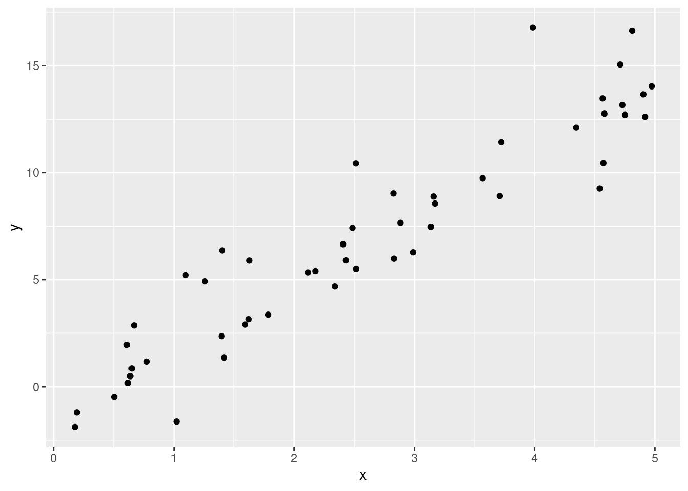
Note that the only source of random variation here is the \(\epsilon\). If \(Y=X\beta\) (without \(\epsilon\)) we would always recover our \(\beta\) coefficient with certainty. But because of \(\epsilon\) can take on certain values, purely due to coincidence, in our sample, this could skew our estimate of \(\beta\), potentially far away from the true \(\beta\). Let me illustrate that with a piece of R code as well:
# Load regression libraries
library(tidyverse, quietly=TRUE); library(fixest, quietly = TRUE); library(modelsummary)

# Reproducible randomness
set.seed(1234)

# Set the parameters
epsilon <- rnorm(n=50, mean=0, sd=2)
beta <- 3
x <- runif(n=50, min=0, max=5)

# Generate Y as a function of X and Epsilon
y <- x*beta + epsilon

# Create a data.frame and plot the data points
df <- tibble(x=x, y=y)

# Plot
ggplot(df, aes(x=x, y=y)) + geom_point()

# Estimate a linear model
feols(y ~ x, data = df) |>
  modelsummary(gof_map = "nobs")
| (1) | |
|---|---|
| (Intercept) | -1.091 |
| (0.505) | |
| x | 3.071 |
| (0.168) | |
| Num.Obs. | 50 |
As you can see, our coefficient estimate is \(3.07\) and not 3, purely due to coincidence in sampling. Hence, our \(\beta\) coefficient also exhibits sampling variation as a result of the randomness in the error term \(\epsilon\).
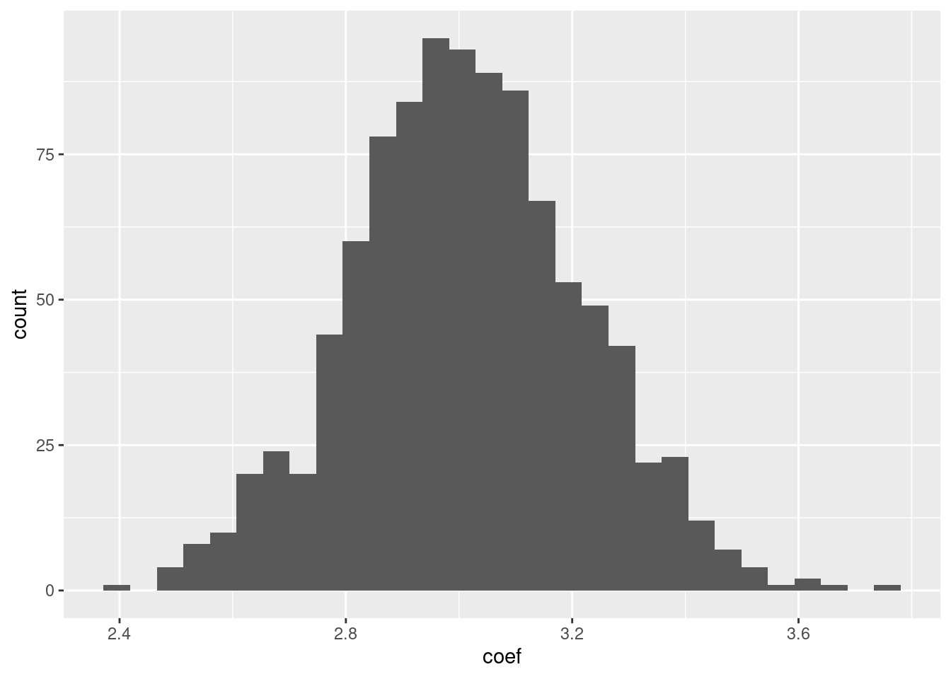
To illustrate that even more clearly, let me repeat the preceding piece of code 1,000 times. That is:
- Sample
\(N=50\)observations from\(\epsilon\)and\(X\). - Generate
\(Y\)from these observations - Estimate the
\(\beta\)coefficient.
And finally, plot the resulting \(1,000 \beta\) coefficients.
coefficients <- map_dbl(1:1000, ~ {
  epsilon <- rnorm(n=50, mean=0, sd=2)
  x <- runif(n=50, min=0, max=5)
  y <- x*beta + epsilon # Remember, true beta is still 3
  df <- tibble(x=x, y=y)
  reg <- feols(y ~ x, data = df)
  estimated_beta <- reg$coeftable$Estimate[2]

  return(estimated_beta)
})

# Plot the result
tibble(coef=coefficients) |>
  ggplot(aes(x=coef)) + geom_histogram()
## `stat_bin()` using `bins = 30`. Pick better value with `binwidth`.

Even though on average, we estimate a \(\beta\) coefficient of 3, but out of these 1,000 times, we have, purely due to coincidental values of our \(\epsilon\) obtained \(\beta\) coefficients that are quite different from 3.
Under the assumption that our error term is normally distributed with mean 0 and variance \(\sigma^2\), we can also derive the sampling distribution for our \(\beta\) coefficients.
Deriving the Sampling Distribution in Linear Regression
Our starting point is a well-known formula for the \(\beta\) coefficients in regression, computed by OLS:
$$ \hat{\beta} = (X^T X)^{-1}X^T y $$
For those unfamiliar with this expression, this is the multivariate expression of the estimated \(\beta\) coefficients. So this allows you to express your \(k\) estimated \(\beta\) coefficients at once. If you haven’t seen this before, don’t worry, it’s just the generalization of the expression \(\hat{\beta}={\text{Cov(X,Y)} \over \text{Var}(X)}\), with the nuance that this expresses all \(k\) \(\beta\) coefficients at once.
What is the distribution of \(\hat{\beta}\)?
Since \(y = X\beta + \epsilon\), substituting this in the expression for \(\hat{\beta}\) gives:
$$ \hat{\beta}= \beta +(X^T X)^{-1}X^T \epsilon $$
We assumed that \(\epsilon\) is normally distributed. Specifically, it is distributed as \(\mathcal{N}(0, \sigma^2 I_n)\) where \(I_n\) is the identity matrix. This is just a very short way of saying that errors are uncorrelated with each other and have constant variance.
Since \(\epsilon\) is a normally distributed variable, a linear function of \(\epsilon\) is also a normally distributed variable.
In fact, this is the generalization of the identity \(\text{Var}(aZ) = a^2 \text{Var}(Z)\) we’ve seen before, but in a multivariate context.
Adding something deterministic, \(\beta\) to that function changes the mean but keeps it a normal variable. Hence, \(\hat{\beta}\) is distributed as:
$$ \hat{\beta} \sim \mathcal{N}(\beta, \sigma^2 (X^T X)^{-1}) $$
In principle, if we knew \(\sigma^2\) (which we don’t, because it’s a population value), we could do hypotheses tests around the \(j\)’th \(\hat{\beta}\) coefficient: we have just argued that \(\beta_j\) is normally distributed with mean \(\beta_j\) and variance \(\sigma^2 (X^T X)^{-1}_{jj}\).
In other words, we have now derived that:
$$ \frac{\hat{\beta}_j - \beta_j}{\text{SE}(\hat{\beta_j})} \sim \mathcal{N}(0,1) $$
where \(\text{SE}(\hat{\beta_j})= \sqrt{\sigma^2 (X^TX)^{-1}_{jj}}\), a result which we obtain by standardizing our variable. SE is short for standard error.
However, the problem is that we don’t know \(\sigma^2\), and we have to estimate it. Estimating it changes the distribution of \(\hat{\beta}\) to a \(t\) distribution rather than a normal distribution. The \(t\) statistics use, instead of \(\text{SE}(\beta_j)\), an estimated standard error, \(\text{SE}_{emp}\), defined as \(\text{SE}_{emp} = \sqrt{\hat{\sigma^2} (X^T X)^{-1}_{jj}}\), with a particular estimate for \(\sigma^2\) motivated in the next section. I have denoted this with \(emp\), short for “empirical”, meaning we use only the data to come up with this estimate. No population parameters are involved. The resulting statistic will be \(t(n-k)\) distributed rather than normally distributed. How that works will also be explained in the next section, but feel free to skip it.
Deriving the \(t\) Distribution
As an estimate of \(\sigma^2\), we’re using the following estimator:
$$ \hat{\sigma^2} = {(\hat{\epsilon}^T \hat{\epsilon}) \over (n-k)} $$
This is an unbiased estimator for \(\sigma^2\) because of the following:
\(\hat{\epsilon}^T \hat{\epsilon} = \epsilon^T M_X \epsilon\), where\(M_X\)is the annihalator matrix. This relates the residuals to the error term.- Using the fact that for a random vector
\(z \sim \mathcal{N}(0, \sigma^2 I_n)\)and an idempotent matrix\(A\)of rank\(r\), the expected value of the quadratic form\(z^T A z = \sigma^2 \cdot \text{tr}(A)\) - Hence the expected value
\(\mathbb{E}[\hat{\epsilon}^T \hat{\epsilon}] = \mathbb{E}[\epsilon^T M_X \epsilon] = \sigma^2 \cdot \text{tr}(M_X)\) - Since the
\(\text{tr}(M_X) = (n-k)\), the expected value\(\mathbb{E}[\hat{\epsilon}^T \hat{\epsilon}] = \sigma^2 (n-k)\), which means that\(\hat{\sigma^2}\)as defined above is unbiased for\(\sigma^2\).
The estimated error variance \(\hat{\sigma^2}\) scaled by the true variance is \(\chi^2\) distributed with \(n-k\) degrees of freedom because of the following:
If
\(A\)is a symmetric, idempotent matrix of rank\(r\), and\(z \sim \mathcal{N}(0,\sigma^2 I_n)\), then\(\frac{z^T A z}{\sigma^2} \sim \chi^2_r\)
Hence in this case,
$$ \frac{(n-k)\hat{\sigma^2}}{\sigma^2} = \frac{\hat{\epsilon}^T \hat{\epsilon}}{\sigma^2} \sim \chi^2_{n-k} \text{ or } \frac{\hat{\sigma^2}}{\sigma^2} \sim \frac{\chi^2_{n-k}}{(n-k)} $$
A \(t\) distribution is defined as
$$
T = \frac{Z}{\sqrt{\frac{V}{v}}}
$$
where \(Z \sim \mathcal{N}(0,1)\) and \(V \sim \chi^2\) with \(v\) degrees of freedom.
Note that our sampling distribution depends on our theoretical distributions as follows:
\begin{align*} \frac{(\hat{\beta}_j - \beta_j)}{SE_{emp} (\beta)} = \frac{\frac{(\hat{\beta}_j - \beta_j)} {\sigma \sqrt{(X^TX)^{-1}_{jj}}}}{\sqrt{\frac{\hat{\sigma^2}}{\sigma^2}}} \end{align*}
This exactly fits the definition of the \(t\) distribution, since \(Z = \frac{(\hat{\beta}_j - \beta_j)} {\sigma \sqrt{(X^TX)^{-1}_{jj}}}\), and the \(\frac{V}{v}\) under the square-root is exactly \(\frac{\hat{\sigma^2}}{\sigma^2}\), which we have seen before, is \(\chi^2\) distributed scaled by its \((n-k)\) degrees of freedom.
Hence, we have proven that under the null hypothesis \(\beta_j\), our \(t\) statistic follows the \(t\) distribution with \((n-k)\) degrees of freedom.
Hypothesis Testing?
So what are we doing when we’re doing hypothesis testing in linear regression? We have now, under certain assumptions, obtained the sampling distribution of our estimated \(\beta\) coefficients. We can use that to impose a null hypothesis of a coefficient \(\beta_j\) taking on a certain value, and consider the sampling distribution. Then, we can compute the likelihood that our coefficient takes on the value of our actually estimated coefficient and, using the sampling distribution, consider how likely such an estimate, or more extreme estimates, are under the null hypothesis.
The resulting likelihood is again defined as the \(p\) value.
The previous expressions allow us to calculate all of this manually. Let’s take a simulate example again and estimate a simple regression:
beta <- 2
data <- tibble(x=runif(20, 1, 5), y = beta*x + rnorm(20, 0, 12))

model <- feols(y ~ x + 0, data = data)
model
## OLS estimation, Dep. Var.: y
## Observations: 20
## Standard-errors: IID
##   Estimate Std. Error t value Pr(>|t|)
## x  2.37497   0.867267 2.73845 0.013058 *
## ---
## Signif. codes:  0 '***' 0.001 '**' 0.01 '*' 0.05 '.' 0.1 ' ' 1
## RMSE: 11.5   Adj. R2: -0.083863
As you can see, our \(\beta\) coefficient is \(2.37\) and our standard error is \(0.86\). Our \(t\) value is \(2.73\) and our \(p\) value about \(0.013\). We have seen before that our (empirical) standard error equals:
$$ \sqrt{\hat{\sigma^2} (X^TX)^{-1}_{jj}} `$$,
which we can also calculate using our data:
n <- 20; k <- 1

# Calculate our estimate sigma_sq_hat
sigma_sq_hat <- 1/(n-k) * model$residuals %*% model$residuals

# Calculate the (empirical) standard error
standard_error <- sqrt(sigma_sq_hat * solve(t(data$x) %*% data$x))
standard_error
##          [,1]
## [1,] 0.867267
.. which is the exact number in the above regression table.
Using this standard error, we can now perform hypothesis tests on our \(\beta\) coefficient. We impose a null hypothesis, for example, that our actual \(\beta\) coefficient equals zero. Then, using the sampling distribution of our coefficient, we can calculate the probability of obtaining the coefficient estimate that we have actually obtained under the null hypothesis:
beta_coefficient <- model$coeftable$Estimate[1]

# Calculate the t-statistic under the null hypothesis that Beta = 0
t_statistic <- beta_coefficient / standard_error
t_statistic
##         [,1]
## [1,] 2.73845
# Calculate the two-sided p-value
p_value <- 2*(1-pt(t_statistic, df = n-1))
p_value
##           [,1]
## [1,] 0.0130577
Where I have calculated the \(p\) value for a two-sided test, reflecting the probability of obtaining the coefficient of obtaining our actually obtained coefficient estimate or something more extreme according to the null hypothesis.
Hence again, the probability of obtaining something like the estimated \(\beta\) coefficient or something more extreme, if the null hypothesis were true, is an event that is extremely unlikely. Hence, we reject the null hypothesis in favor of the alternative hypothesis.
Note, finally, that the \(t\) statistic and \(p\) value are exactly equal to those in the regression table.
Hypothesis Testing Graphically
To close off this post, let me demonstrate the process of testing
$$ H_0: \beta = 0 \ H_A: \beta \neq 0 $$
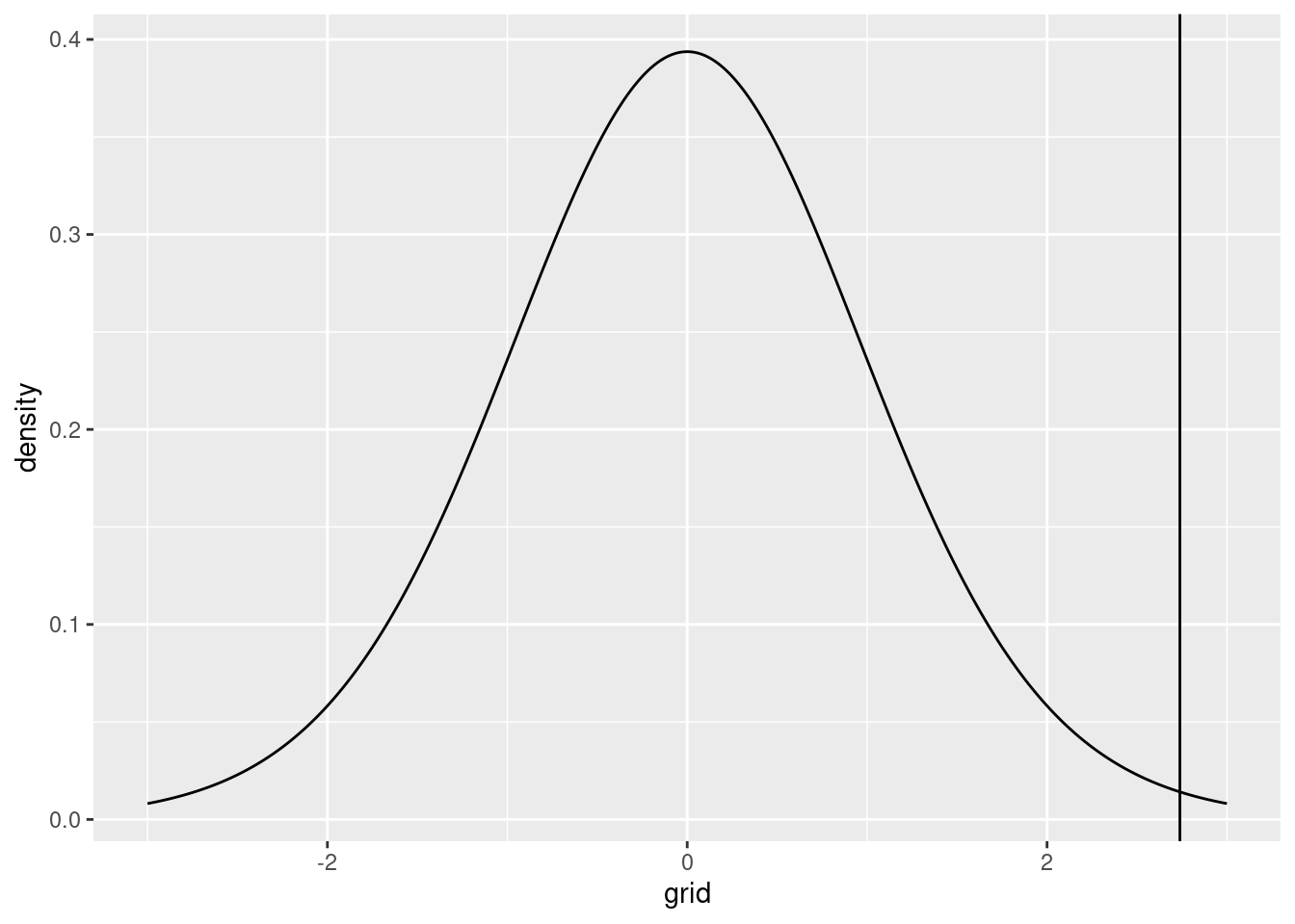
.. And let’s do this graphically. Under the null hypothesis, \(\beta\) is \(t\) distributed with \(n-k\) degrees of freedom, which in our example amounted to \(20 -1 = 19\) degrees of freedom. Hence, the distribution of \(t\) statistics under the null hypothesis looks as follows:
t_dist <- tibble(grid=seq(-3, 3, by=0.01), density=dt(grid,df = n-k))
p1 <- t_dist |>
  ggplot(aes(x=grid, y=density)) + geom_line()

p1

Our obtained \(t\) statistic, however, was equal to 2.7384503. Graphically:
p2 <- p1 + geom_vline(xintercept=t_statistic)

p2

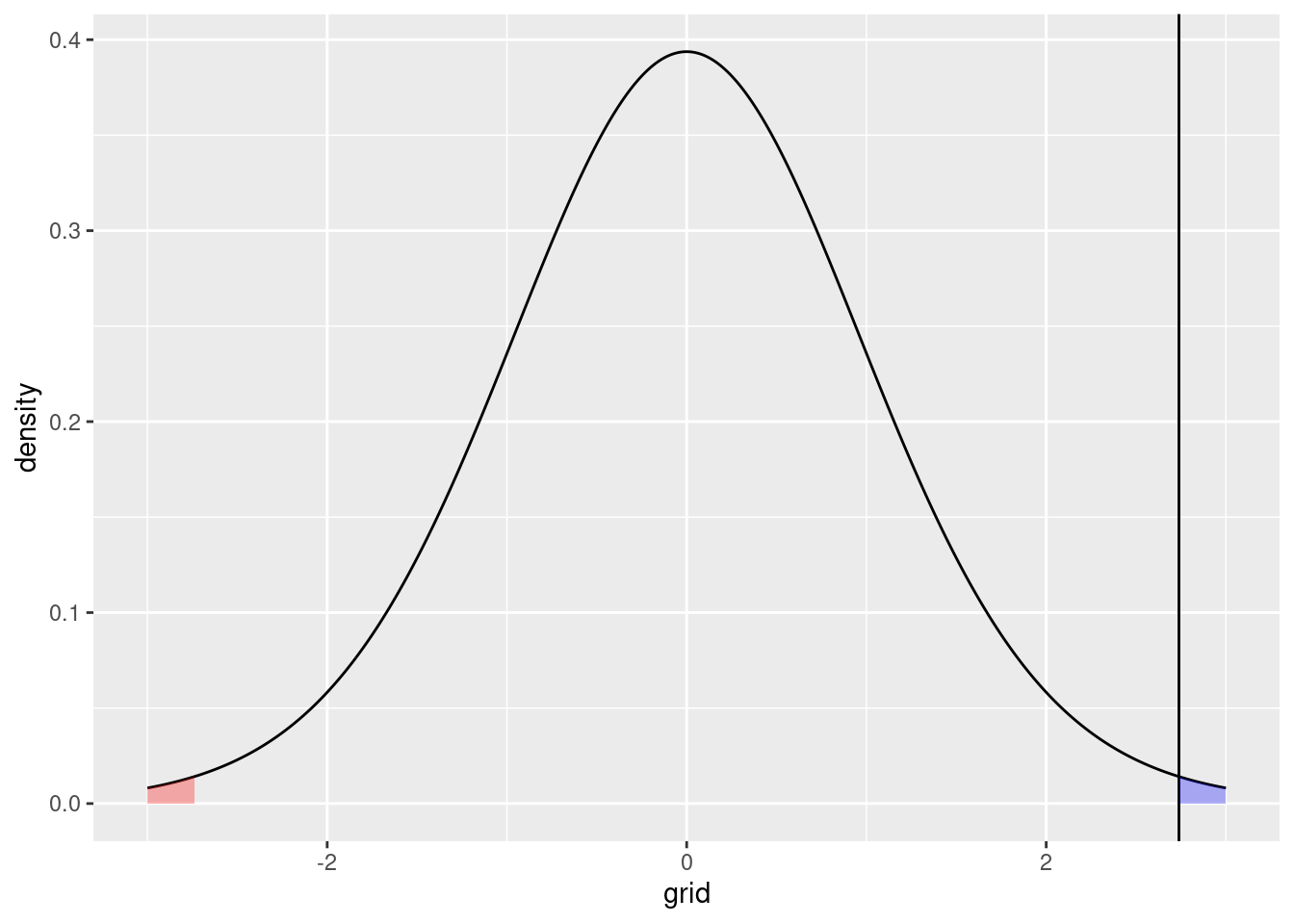
This is an extremely unlikely event under the null hypothesis. The \(p\) value can also be visualized by showing the probability under the null hypothesis of obtaining our actual \(t\) value or something more extreme:
right_tail <- t_dist |> filter(grid >= as.numeric(t_statistic))
left_tail <- t_dist |> filter(grid < -as.numeric(t_statistic))
p2 + geom_area(data = right_tail,
               aes(x = grid, y = density),
               fill = "blue",
               alpha = 0.3) +
  geom_area(data = left_tail,
            aes(x = grid, y = density),
            fill= "red",
            alpha = 0.3)

The one-sided \(p\) value corresponding to the blue area, and the two-sided \(p\) value, as reported here, corresponding to the combined blue and red areas.
Conclusion
This blog post focused on the concept of sampling variation. In part I, in a very simple case, we introduced the concept by looking at a series of \(N\) i.i.d. normal variables, and derived the uncertainty surrounding our estimated mean.
Then, we did the same thing for linear regression, which turned out to be a little bit more difficult. The difficulty was that we don’t have access to the error variance parameter \(\sigma^2\), but have to make do with an estimate of that parameter. That makes it that the final sampling distribution we end up with is not normal, but \(t\) distributed.
Finally, we focused on hypothesis testing. In hypothesis testing, we hold that the true coefficient estimate is a certain number, for example, 0. Then, we use our obtained information on the sampling distribution to consider how likely it is that our actual coefficient has been obtained given that the true coefficient is zero, and the sampling distribution is the distribution we’ve estimated.
Hopefully, this background article has helped you visualizing and seeing more clearly how sampling variation, and its conceptual sibling, hypothesis testing, work. Thanks for reading! If you have any comments, mail them to a dot h dot machielsen at uu dot nl.
- Posted on:
- October 8, 2024
- Length:
- 10 minute read, 2099 words
- See Also: