The Besley and Case (1995) Model

Introduction

Besley and Case (1995) have a paper about the influence of term limits for politicians on policy behavior. They use a dynamic game. Politicians can serve either one or two periods, depending on whether they are retained. In these periods, politicians choose to put in effort. Putting in more or less effort is costly to different extents, according to their type. The chosen effort probabilistically affects a policy outcome. An infinitely-lived voter makes decisions to retain or dismiss the politician after observing the outcome. Their solution, based on Banks and Sundaram (1998) involves a cut-off equilibrium, with voters reelecting an incumbent politician if the probabilistically-influenced policy variable realization is higher than some threshold \(r_{min}\).

One of their key predictions is that the equilibrium amount of effort put in by politicians in their first period is higher than in their last period, irrespective of the politician’s type. The model predicts that the prospect of re-election incentivizes politicians to exert higher effort. Consequently, politicians in their first term will, on average, exert more effort and produce better policy outcomes than they will in their final term, when re-election is no longer a motivation. As Besley and Case put it:

If two terms are allowed, then incumbents who give higher first-term payoffs to voters are more likely to be retained to serve a second term. Those in their last term put in less effort and give lower payoffs to voters, on average, compared with their first term in office.

Their model is fairly general, so in this blog post, I wanted to give an easier-to-understand version for a specific case using Python to solve for some expressions that are not analytically soluble. I also want to demonstrate how to use standard computational techniques for this specific case.

Set-up

In the Besley and Case (1995) model, there can be \(k\) types of politicians, ordered by ability \(\omega_1 < \dots < \omega_k\). They occur with probabilities \(\pi_1, \dots, \pi_k\). In my setup, there are only two types, \(\omega_1 < \omega_2\) with \(\omega_1 = 3\) and \(\omega_2 = 9\). \(\omega_1\) occurs with probability \(\pi_1 = 0.2\) and \(\omega_2\) with probability \(\pi_2 = 0.8\). The politician’s per-period utility is:

\[ v(\alpha, \omega_i) = \alpha - \frac{\alpha^2}{\omega_i} \]

If the politician is in power, otherwise, utility is zero. This reflects a reward proportional to effort, while effort is also costly (utility is quadratic in effort), with the cost being lower for higher-quality types.

Effort is mapped into policy outcomes, \(r\), probabilistically via \(F(\alpha, r)\). In the Besley and Case (1995) setting, this can be any distribution satisfying the monotone likelihood ratio property. In my setting, I take the outcome distribution to be Normal, meaning \(R \sim \mathcal{N}(\alpha, 1)\). The voter’s one-period utility is simply the realized outcome \(r\).

Optimization of the politician

In the second (and final) period, the politician faces no re-election incentive and will simply optimize their one-period utility by choosing effort \(\alpha\): \[ \max_{\alpha} \left( \alpha - \frac{\alpha^2}{\omega_i} \right) \]

The first-order condition is \(1 - \frac{2\alpha}{\omega_i} = 0\), which yields the optimal second-period effort:

\[ a^s_i = \frac{\omega_i}{2} \]

In the first period, the politician chooses effort to maximize their current utility plus the discounted expected utility from a potential second term:

\[ a^l_i = \arg\max_{\alpha} \left\{ v(\alpha, \omega_i) + \delta \cdot \text{Pr}(\text{re-election} | \alpha) \cdot v(a^s_i, \omega_i) \right\} \]

Given the voter’s retention rule, the probability of re-election is the probability that the realized outcome \(r\) is greater than the voter’s retention threshold, \(\text{Pr}(r > r_{\min} | \alpha)\).

Optimization of the voter

After observing the realized outcome \(r\) after one period, the voter updates their belief that the incumbent is the low type (\(\omega_1\)) using Bayes’ rule:

\[ \beta_1(r) = \frac{\pi_1 \cdot f(r | a^l_1)}{\pi_1 \cdot f(r | a^l_1) + \pi_2 \cdot f(r | a^l_2)} \]

The expected utility to the voter of retaining the incumbent for a second period is the belief-weighted average of the expected outcomes from each type’s second-period effort:

\[ v_2(r) = \beta_1(r) \cdot E[\hat{r} | a^s_1] + (1 - \beta_1(r)) \cdot E[\hat{r} | a^s_2] \]

Since utility is linear in \(r\) and \(E[\hat{r} | a^s_i] = a^s_i\), this simplifies to:

\[ v_2(r) = \beta_1(r) \cdot a^s_1 + (1 - \beta_1(r)) \cdot a^s_2 \]

Banks and Sundaram (1993) show that the Bellman equation for the voter’s problem when facing an incumbent who has served one term is:

\[ W(1, r, p) = \max \left\{ v_2(r) + \delta W(0, \pi), W(0, \pi) \right\} \]

The first term inside the max is the value of retaining the incumbent, and the second is the value of dismissing them and drawing a new politician. The state vector is {term, r, beliefs}. Here, term=1 means the incumbent can serve one more term. \(W(0, \pi)\) represents the value of drawing a new politician, where beliefs are reset to the prior probabilities \(\pi\).

The Bellman equation for the state \(W(0, \pi)\), the value of drawing a fresh politician, is the expected immediate reward from that new politician’s first term, plus the discounted continuation value:

\[ W(0, \pi) = \sum_{i=1}^2 \pi_i \cdot E[\hat{r} | a^l_i] + \delta \int W(1, \hat{r}, \beta_1(\hat{r})) \left( \sum_{k=1}^2 \pi_k \cdot f(\hat{r} | a^l_k) \right) d\hat{r} \]

Note that the efforts used here must be the first-period efforts, \(a^l_k\), as this state represents the start of a new politician’s potential two-term tenure. So what is this? In simple terms, \(W(0, \pi)\) is the voter’s total expected lifetime utility from the moment they decide to bring in a new, unknown politician.

This situation arises in two scenarios:

1. The voter dismisses an incumbent after their first term.
2. An incumbent has finished their second and final term, and a new election must be held.

The equation defines this value recursively, following the fundamental principle of dynamic programming: “The value of a decision today is the immediate reward you get plus the discounted value of the best situation you can be in tomorrow.”

• \(W(...)\): This is the Value Function. It represents the maximum expected lifetime utility for the voter, starting from a specific state.
• \(0\): This is the first element of the state vector, representing the number of re-election terms an incumbent has remaining. A \(0\) here signifies that we are not evaluating an incumbent. Instead, we are at a “clean slate” moment—the value of drawing a new politician who will start their first term.
• \(\pi\): This represents the voter’s beliefs. Since the politician is a fresh draw from the pool of candidates, the voter has no performance information yet. Their belief about the politician’s type is simply the objective prior probability distribution, \(\pi = (\pi_1, \pi_2)\) (e.g., a 20% chance of being low-ability, 80% chance of being high-ability).

So, \(W(0, \pi)\) reads as “The value to the voter of being in a state where a new politician is about to be drawn, and beliefs about this politician are the priors \(\pi\).”

The RHS is composed of two main parts, representing “what I get now” and “what I get later.”

\[ \sum_{i=1}^2 \pi_i \cdot E[\hat{r} | a^l_i] \]

This term calculates the expected utility the voter will receive in the very next period from this new politician.

• \(\pi_i\): The probability that the new politician is of type \(i\).
• \(a^l_i\): The optimal first-period effort that a politician of type \(i\) will exert. It is critically important that this is \(a^l\) (first-period effort) and not \(a^s\) (second-period effort), because this new politician has a re-election incentive and will adjust their behavior accordingly.
• \(E[\hat{r} | a^l_i]\): The expected policy outcome \(\hat{r}\) (and thus the voter’s expected utility, since it’s linear) given that the politician exerts effort \(a^l_i\). In the specific model where \(r \sim \mathcal{N}(\alpha, 1)\), this expected value is simply \(a^l_i\).
• \(\sum\) (Summation): The voter doesn’t know the type of the new politician. The summation takes the average of the expected outcomes, weighted by the probability of drawing each type.

The voter thinks, “With probability \(\pi_1\), I’ll get a low-ability politician who will give me an expected outcome of \(a^l_1\). With probability \(\pi_2\), I’ll get a high-ability politician who will give me \(a^l_2\). My expected utility for this first period is the average of those two possibilities.”

\[ \delta \int W(1, \hat{r}, \beta_1(\hat{r})) \left( \sum_{k=1}^2 \pi_k \cdot f(\hat{r} | a^l_k) \right) d\hat{r} \]

This term represents the value of all subsequent periods, starting from the period after the new politician’s first term.

• \(\delta\): The voter’s discount factor (\(0 < \delta < 1\)). Future utility is worth less than present utility, and \(\delta\) captures this time preference.

• \(\int \dots d\hat{r}\) (The Integral): The voter knows that some outcome \(\hat{r}\) will be realized, but they don’t know what it will be. The integral sums up the value across all possible continuous outcomes \(\hat{r}\), weighting each by its probability of occurring.

Let’s break down the two components inside the integral:

1. The Future Value \(W(1, \hat{r}, \beta_1(\hat{r}))\):
   • This is the value of the state the voter will be in after observing the outcome \(\hat{r}\).
   • \(1\): The state has transitioned. The politician has served one term and now has one re-election term remaining.
   • \(\hat{r}\): The specific outcome that was realized. This is now known history and is part of the new state.
   • \(\beta_1(\hat{r})\): The voter’s updated belief (the posterior probability) that the politician is low-ability, calculated using Bayes’ rule after observing \(\hat{r}\). A high \(\hat{r}\) will lower this belief, making the voter more optimistic about the incumbent. The future value heavily depends on this belief.
2. The Probability Weight \(( \sum_{k=1}^2 \pi_k \cdot f(\hat{r} | a^l_k) )\):
   • This term is the probability density function of observing the outcome \(\hat{r}\). It’s the overall likelihood of a specific \(\hat{r}\) happening.
   • It’s calculated using the Law of Total Probability: The total probability of seeing \(\hat{r}\) is (the probability of drawing type 1 \(\times\) the probability that type 1 produces \(\hat{r}\)) + (the probability of drawing type 2 \(\times\) the probability that type 2 produces \(\hat{r}\)).

The voter thinks, “After the first period, some outcome \(\hat{r}\) will occur. For any given \(\hat{r}\), I’ll update my beliefs and be faced with a new problem: whether to keep or dismiss this incumbent, a state which has value \(W(1, \hat{r}, \beta_1(\hat{r}))\). To find the expected value of the future, I must average the values of all these possible future states, weighting each by the probability that the \(\hat{r}\) leading to it actually happens. Finally, I’ll discount this entire future prospect by \(\delta\).”

Putting it all together, the Bellman equation \(W(0, \pi)\) establishes the “outside option” or “reset value” for the voter. Whenever the voter considers dismissing an incumbent, they compare the value of keeping them against the value of starting fresh, which is exactly \(W(0, \pi)\).

Now that we have the Bellman equations, we can use value-function iteration to find the voter’s optimal retention rule.

Implementation

Below, I load the necessary libraries and define a Python class RetentionModel to hold the model’s parameters and methods.

#%matplotlib inline
import matplotlib.pyplot as plt
plt.rcParams["figure.figsize"] = (11, 5)  #set default figure size
import numpy as np
from interpolation import interp
from scipy.optimize import minimize_scalar
from scipy.stats import norm
import scipy.interpolate as interpolate

class RetentionModel:
  
    def __init__(self, delta=0.95, types=(3, 9), types_freq=(0.2, 0.8)):
        self.delta, self.types, self.types_freq = delta, types, types_freq
    
        # Create a 3-dimensional grid for the state space: {term, r, belief}
        self.x_grid = np.mgrid[0:2, 2.5:3.5:0.1, 0:1.05:0.1].reshape(3, -1).T
        
    def f(self, r, effort):
        """Normal PDF of r given exerted effort."""
        return norm.pdf(r, loc=effort, scale=1)
    
    def F(self, r, effort):
        """Normal CDF of r given exerted effort."""
        return norm.cdf(r, loc=effort, scale=1)

    def expected_utility_politician(self, effort, typ, retention_r):
        """
        Politician's total expected utility from the first period, looking forward.
        """
        # Utility from period 1 + discounted expected utility from period 2
        v_s = self.effort_second_period(typ) - (self.effort_second_period(typ)**2) / typ
        out = effort - (effort**2) / typ + self.delta * (1 - self.F(retention_r, effort)) * v_s
        return out

    def effort_first_period(self, typ, retention_r):
        """Optimal effort in the first period given type."""
        res = maximize(self.expected_utility_politician, 1e-15, typ, (typ, retention_r))
        return res[0]

    def effort_second_period(self, typ):
        """Optimal effort in the second period given type."""
        return typ / 2
    
    def beta_1(self, r, retention_r):
        """
        Voter's posterior belief that politician is type 1 after observing r.
        """
        types, types_freq, f = self.types, self.types_freq, self.f
        
        # Calculate first period efforts based on the current retention rule
        a1_l = self.effort_first_period(types[0], retention_r)
        a2_l = self.effort_first_period(types[1], retention_r)
        
        num = types_freq[0] * f(r, a1_l)
        denom = num + types_freq[1] * f(r, a2_l)
        
        # Handle cases where denom is zero to avoid division by zero
        return np.divide(num, denom, out=np.full_like(num, types_freq[0]), where=denom!=0)

    def v_2(self, r, retention_r):
        """
        Voter's expected utility from retaining the incumbent for a second period.
        """
        beta1_r = self.beta_1(r, retention_r)
        
        eff_sp_t1 = self.effort_second_period(self.types[0])
        eff_sp_t2 = self.effort_second_period(self.types[1])
        
        # E[r|a] = a since r ~ N(a, 1) and voter utility is linear
        expected_utility = beta1_r * eff_sp_t1 + (1 - beta1_r) * eff_sp_t2
        return expected_utility
    
    def state_action_value(self, action, state, v_array, retention_r):
        """
        Calculates the value of taking an action given a state and a guess for the value function.
        """
        types, types_freq, delta, f = self.types, self.types_freq, self.delta, self.f
        
        # Create a multi-dimensional linear interpolator for the value function
        v_func = interpolate.LinearNDInterpolator(self.x_grid, v_array, fill_value=0)
        
        # State: {term, r, belief}
        term = state[0]
        
        if term == 0: # Value of drawing a new politician
            a1_l = self.effort_first_period(types[0], retention_r)
            a2_l = self.effort_first_period(types[1], retention_r)
            
            # Expected immediate reward from a new politician's first term
            immediate_reward = types_freq[0] * a1_l + types_freq[1] * a2_l
            
            # Define the integrand for the continuation value
            def integrand(r_hat):
                # Probability density of a given r_hat occurring
                prob_r_hat = types_freq[0] * f(r_hat, a1_l) + types_freq[1] * f(r_hat, a2_l)
                # Updated belief
                beta1_r_hat = self.beta_1(r_hat, retention_r)
                # Value of being in state (1, r_hat, beta1_r_hat)
                future_val = v_func([1, r_hat, beta1_r_hat])[0]
                return future_val * prob_r_hat

            # A simple numerical integration (quadrature)
            r_range = np.linspace(0, 13, 100)
            integral_values = np.array([integrand(r) for r in r_range])
            continuation_value = np.trapz(integral_values, r_range)
            
            return immediate_reward + delta * continuation_value
        
        elif term == 1: # Value for an incumbent
            w0 = v_func([0, state[1], types_freq[0]])[0] # Value of dismissing
            
            if action == "k": # Keep
                return self.v_2(state[1], retention_r) + delta * w0
            
            elif action == "d": # Dismiss
                return w0
            
            else:
                raise ValueError("No action chosen")

I also define a custom maximizer to handle the voter’s discrete choice ({retain, dismiss}) and a continuous maximizer for the politician’s effort choice.

def maximize(g, a, b, args):
    """
    Maximize the function g over the interval [a, b].
    """
    objective = lambda x: -g(x, *args)
    result = minimize_scalar(objective, bounds=(a, b), method='bounded')
    maximizer, maximum = result.x, -result.fun
    return maximizer, maximum

def maximize_sav(function, args):
    """
    Maximizes the state-action value for a given state over the discrete actions {k, d}.
    """
    state, v_array, retention_r = args
    
    if state[0] == 0:
        # If term is 0, there is no incumbent, so the only "action" is drawing a new politician
        action = "d" # Represents drawing a new politician
        maximum = function("d", state, v_array, retention_r)
    elif state[0] == 1:
        dismiss_val = function("d", state, v_array, retention_r)
        keep_val = function("k", state, v_array, retention_r)
        if dismiss_val > keep_val:
            action = "d"
            maximum = dismiss_val
        else:
            action = "k"
            maximum = keep_val
        
    return action, maximum

Value Function Iteration

Then, I instantiate the model and apply value function iteration to solve for the voter’s optimal policy and value function.

model = RetentionModel(delta=0.95)

def T(v, rm, retention_r):
    """
    The Bellman operator. Updates the guess of the value function.
    """
    v_new = np.empty_like(v)
    policy_new = [None] * len(v_new)

    for i, x in enumerate(rm.x_grid):
        sol = maximize_sav(rm.state_action_value, args=(x, v, retention_r))
        policy_new[i] = sol[0]
        v_new[i] = sol[1]
    
    # Find the lowest r on the grid where the optimal action is to 'keep'
    try:
        # Filter for states where term=1
        incumbent_indices = [i for i, state in enumerate(rm.x_grid) if state[0] == 1]
        # Find the first index among these where the policy is 'k'
        first_keep_index = next(i for i in incumbent_indices if policy_new[i] == 'k')
        new_retention_r = rm.x_grid[first_keep_index][1]
    except StopIteration:
        # If 'k' is never chosen, set the threshold to a very high number
        new_retention_r = 1e6

    return policy_new, v_new, new_retention_r

def compute_value_function(rm, tol=1e-4, max_iter=200, verbose=True, print_skip=5):
    """
    Iteratively solves for the value function.
    """
    v = np.zeros(len(rm.x_grid)) # Initial guess for value function
    rr = 3.0 # Initial guess for retention rule
    
    i = 0
    error = tol + 1

    while i < max_iter and error > tol:
        policy_new, v_new, rr_new = T(v, rm, rr)
        
        error = np.max(np.abs(v - v_new))
        i += 1

        if verbose and i % print_skip == 0:
            print(f"Iteration {i}: error = {error:.6f}, new r_min = {rr_new:.4f}")

        v = v_new
        rr = rr_new

    if i == max_iter:
        print("Failed to converge!")

    if verbose and i < max_iter:
        print(f"\nConverged in {i} iterations.")

    return policy_new, v_new, rr_new

Solution

The procedure converges and the model is solved.

out = compute_value_function(model)

/tmp/ipykernel_172580/523693392.py:96: DeprecationWarning: `trapz` is deprecated. Use `trapezoid` instead, or one of the numerical integration functions in `scipy.integrate`.
  continuation_value = np.trapz(integral_values, r_range)

Iteration 5: error = 0.025946, new r_min = 2.5000
Iteration 10: error = 0.000142, new r_min = 2.5000

Converged in 11 iterations.

The optimal retention rule \(r_{\min}\) for this specific case is:

print(f"The optimal retention threshold r_min is: {out[2]}")

The optimal retention threshold r_min is: 2.5

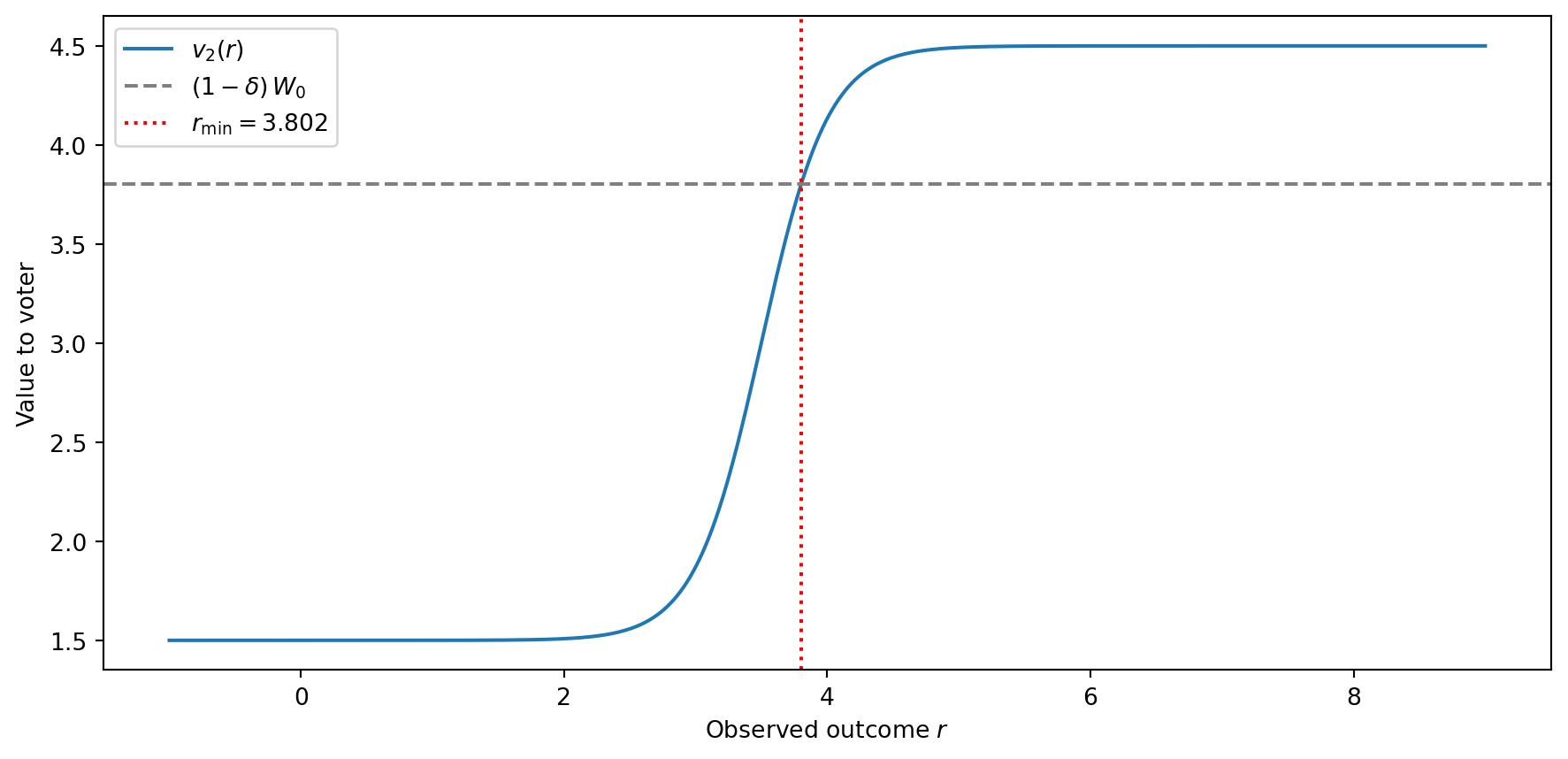
This is an interior solution to the problem. It is also easily verifiable that this solution characterizes a cut-off rule, as described by Banks and Sundaram (1993), where the voter retains the incumbent if and only if the observed outcome \(r\) is above this threshold.

I hope this has been useful! If you have any tips or remarks, let me know, and thanks for reading.