Spectral Clustering Polygons into Macroregions

Introduction

In this blog post, I want to show how to use spectral clustering, an unsupervised machine learning algorithm, to cluster polygons into macroregions. An application of this method of clustering might be to aggregate from the city/municipality level up to a higher level, but not the province level (which is something likely to already be in your shapefile). This gives a researcher the opportunity to combine observations from different, but geographically close cities. This method of clustering has several advantages:

• It can discover clusters of arbitrary shape.
• It’s not as sensitive to the initial configuration as some other clustering algorithms.
• It can incorporate additional features or similarity measures into the clustering process, as shown in the previous responses.

Formulation of the algorithm

Step 1: Compute the Similarity Matrix

You start by creating a similarity matrix \(S\), where \(S_{ij}\) represents the similarity between data points \(x_i\) and \(x_j\). In the setting I will explain below, this similarity matrix is the adjacency matrix:

\[ S_{ij} = \begin{cases} 1 & \text{if Municipality $i$ borders Municipality $j$ and Region $i$ = Region $j$} \\\ 0 & \text{otherwise} \end{cases} \]

However, the similarity can also be defined using various other metrics like Gaussian similarity, \(k\)-nearest neighbors, or other similarity measures. A lot of more nuanced methods come from a good definition of the similarity matrix. For example, in the application that follows, I never want to cluster two municipalities from different provinces together. Hence this definition. In another application, I might want to cluster municipalities together if both of their populations are relatively small, whereas I might want to leave them alone if not.

Step 2: Create the Graph Laplacian Matrix

Next, you construct a graph Laplacian matrix, also called the affinity matrix \(L\), from the similarity matrix \(S\). There are different ways to define the Laplacian matrix, but a common choice is the normalized Laplacian, which is defined as:

\[ L=I- D^{−1/2} SD^{−1/2} \]

Where:

• \(I\) is the identity matrix.
• \(D\) is a diagonal matrix with \(D_{ii}=\sum_j S_{ij}\).

This matrix is called the affinity matrix since the distance \(\approx\) 1 - affinity, and the diagonal matrices make sure that distances are normalized between 0 and 1.

Step 3: Compute the eigendecomposition of the \(L\) Matrix.

\(L\), an \(n \times n\) matrix, can be decomposed according to the eigencomposition, say in the matrices \(\Gamma \Omega \Gamma\), where \(\Gamma\) is the matrix of (normalized) eigenvectors of \(L\).

Step 4: Use a clustering algorithm on the eigenvector matrix

Now, take the first \(k\) eigenvectors (corresponding to the lowest \(k\) eigenvalues). Considering the interpretation of this decomposition as a kind of principal component analysis, this accomplishes that observations are as different as possible for a given number of \(k\) eigenvectors: the last \(n-k\) eigenvectors (corresponding to the largest eigenvalues) are responsible for the main bulk of the variance. On these \(k\) eigenvectors, use a clustering algorithm such as k-means.

Example: clustering Dutch Municipalities into Macroregions

I will provide an example of spectral clustering in Python. For this, I use a .geojson file of the Netherlands consisting of polygons of all municipalities. It is available here.

First, I load the relevant packages, after which I make a slight correction to the GeoDataFrame. The most important part is calculating the \(n \times n\) similarity matrix: the elements on the diagonal are naturally 1, since a polygon is similar to itself, and on the off-diagonal, I decide that polygons are similar if they border each other.

Afterwards, I use the similarity matrix to calculate a normalized “Laplacian”, or affinity matrix (denoted by \(L\) in the above). Similarities here are scaled by the “total similarity” to other polygons in the data frame.

import geopandas as gpd
import numpy as np
import pandas as pd  # Import pandas for concatenation
from sklearn.cluster import SpectralClustering
import matplotlib.pyplot as plt

# Retrieve data with municipal boundaries
url = 'https://datasets.iisg.amsterdam/api/access/datafile/9603'
gdf = gpd.read_file(url)

# Fix invalid geometries
gdf['geometry'] = gdf['geometry'].buffer(0)

# Calculate pairwise similarity based on the spatial relationship
similarity_matrix = np.zeros((len(gdf), len(gdf)))

for i in range(len(gdf)):
    for j in range(i, len(gdf)):  # Optimization: only compute upper triangle
        if i == j:
            similarity_matrix[i][j] = 1
        elif gdf.iloc[i].geometry.touches(gdf.iloc[j].geometry):
            similarity_matrix[i][j] = 1
            similarity_matrix[j][i] = 1 # Explicitly make it symmetric

# Note: Normalization is often not necessary if you are just using adjacency (0s and 1s).
# The raw similarity_matrix can be used directly as the affinity matrix.
# If you do need to normalize, ensure the method preserves symmetry.

# --- Perform spectral clustering ---
n_clusters = 12  # Number of macro polygons

# Use the symmetric similarity_matrix directly
clustering = SpectralClustering(
    n_clusters=n_clusters,
    affinity='precomputed',
    assign_labels='discretize'
).fit(similarity_matrix)

/home/bas/Documents/git/website/.venv/lib/python3.10/site-packages/sklearn/manifold/_spectral_embedding.py:328: UserWarning: Graph is not fully connected, spectral embedding may not work as expected.
  warnings.warn(

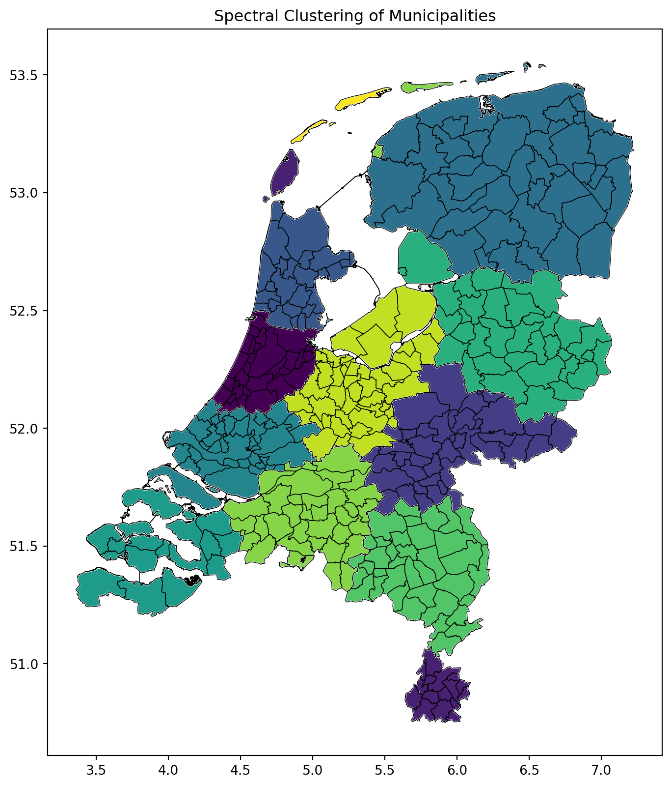
Now, after clustering has finished (I require 12 clusters), we create a new GeoDataFrame to store our new macroregions, that is, merge the polygons within each cluster to create macro polygons.

Finally, in what follows, I plot the new macropolygons next to the original:

# Post-processing: Merge polygons based on cluster labels

# Create a list to hold the new geometries
new_polygons = []

# Iterate through the clusters
for cluster_id in range(n_clusters):
    # Extract polygons in the current cluster
    cluster_mask = (clustering.labels_ == cluster_id)
    cluster_gdf = gdf[cluster_mask]
    
    if not cluster_gdf.empty:
        # Merge polygons within the cluster using the correct method
        merged_polygon = cluster_gdf.union_all()

        # Add the merged polygon to our list
        new_polygons.append(merged_polygon)

# Create the final GeoDataFrame from the list of merged polygons
# This is the correct way to build a GeoDataFrame in a loop
macro_polygons = gpd.GeoDataFrame(geometry=new_polygons, crs=gdf.crs)

# Plotting the result ---
fig, ax = plt.subplots(1, 1, figsize=(10, 10))
macro_polygons.plot(ax=ax, cmap='viridis', edgecolor='white')
gdf.boundary.plot(ax=ax, color='black', linewidth=0.5) # Original boundaries for context
ax.set_title("Spectral Clustering of Municipalities")
plt.show()

Conclusion

Spectral Clustering is a powerful clustering method suitable for clustering polygons into macropolygons, pixels into macropixels, etc. By defining the distance matrix ourselves, we have seen that it can be quite powerful and customizable to accomplish the kind of clusters you want. I hope you found this demonstration useful, and thank you for reading!