Storey’s \(q\) Values and The Bonferroni Correction
Author
Bas Machielsen
Published
November 6, 2025
Introduction
When dealing with a multitude of simultaneous hypothesis tests, the concepts of q-values, Storey’s method, and the Bonferroni correction are crucial for controlling error rates. While both aim to address the issue of multiple comparisons, they do so from different perspectives, offering a trade-off between statistical power and the type of error being controlled. This document will delve into the mathematical underpinnings of these methods, contrast their approaches, and provide a practical guide to their implementation in R.
When conducting multiple hypothesis tests, the probability of making a Type I error—incorrectly rejecting a true null hypothesis—inflates. For instance, if you perform 100 tests with a significance level (alpha) of \(0.05\), you would expect to see 5 false positives by chance alone. To counter this, various correction methods have been developed.
Bonferroni Correction: Controlling the Family-Wise Error Rate (FWER)
The Bonferroni correction is a straightforward and widely used method that controls the Family-Wise Error Rate (FWER). The FWER is the probability of making at least one Type I error among all the hypotheses tested. The Bonferroni correction achieves this control by adjusting the significance level for each individual test. The formula is simple:
Adjusted alpha = \(\frac{\alpha}{m}\)
Where:
\(\alpha\) is the desired overall significance level (e.g., 0.05).
\(m\) is the total number of hypothesis tests being performed.
A p-value is then considered statistically significant only if it is less than or equal to this new, more stringent adjusted alpha.
Alternatively, and more commonly in software packages, the p-values themselves are adjusted. The Bonferroni-adjusted p-value is calculated as:
\(p_{adjusted} = p_{original} \times m\)
If the adjusted p-value exceeds 1, it is set to 1. A hypothesis is rejected if its adjusted p-value is less than the original alpha.
The mathematical proof for the Bonferroni correction’s control of the FWER relies on Boole’s inequality, which states that for a set of events, the probability of at least one of them occurring is no greater than the sum of their individual probabilities.
Click to see the proof.
We want to prove that for a family of \(m\) hypothesis tests, applying the Bonferroni correction ensures that the probability of making one or more Type I errors (the FWER) is less than or equal to a desired significance level \(\alpha\):
FWER \(\le \alpha\)
1. Definitions and Setup
Let there be \(m\) null hypotheses, \(H_1, H_2, \dots, H_m\).
Let \(p_1, p_2, \dots, p_m\) be the corresponding p-values for these tests.
Let \(m_0\) be the number of these null hypotheses that are actually true.
A Type I error occurs if we reject a true null hypothesis.
The Family-Wise Error Rate (FWER) is the probability of making at least one Type I error. FWER = \(P(\text{reject at least one true } H_i)\)
The Bonferroni correction rejects the null hypothesis \(H_i\) if its p-value \(p_i \le \frac{\alpha}{m}\).
2. The Proof Using Boole’s Inequality
Let \(A_i\) be the event that a true null hypothesis \(H_i\) is incorrectly rejected. By the definition of a p-value, under a true null hypothesis, the probability of observing a p-value less than or equal to some value \(x\) is \(x\). That is, \(P(p_i \le x | H_i \text{ is true}) = x\).
Therefore, the probability of making a Type I error for a single true null hypothesis \(H_i\) using the Bonferroni-corrected threshold is:
The FWER is the probability of at least one of these events \(A_i\) occurring for the \(m_0\) true null hypotheses. This can be written as the probability of the union of these events:
Now, we apply Boole’s inequality. Boole’s inequality states that for any finite or countable set of events, the probability that at least one of the events happens is no greater than the sum of the probabilities of the individual events.
We can now substitute the probability of each individual event \(A_i\) into this inequality:
FWER \(\le \sum_{i=1}^{m_0} \frac{\alpha}{m}\)
This is the sum of \(\frac{\alpha}{m}\) added together \(m_0\) times:
FWER \(\le m_0 \cdot \frac{\alpha}{m}\)
Since the number of true null hypotheses (\(m_0\)) is, by definition, less than or equal to the total number of hypotheses (\(m\)), we have \(m_0 \le m\). Therefore:
FWER \(\le m_0 \cdot \frac{\alpha}{m} \le m \cdot \frac{\alpha}{m}\)
This simplifies to:
FWER \(\le \alpha\)
3. Conclusion
This completes the proof. We have shown that by setting the significance threshold for each individual test to \(\frac{\alpha}{m}\), the probability of making at least one Type I error across the entire family of tests is controlled at a level no greater than \(\alpha\). This holds regardless of how many of the null hypotheses are true and whether the tests are independent or not.
Controlling the False Discovery Rate (FDR)
In many research fields, especially those involving large-scale data, controlling the FWER can be overly conservative, leading to a high number of false negatives (failing to reject a false null hypothesis). An alternative approach is to control the False Discovery Rate (FDR), which is the expected proportion of false positives among all the rejected hypotheses. Storey’s method introduces the concept of the \(q\)-value to achieve this.
Mathematical Concept of the q-value
The q-value for a particular hypothesis test is the minimum FDR that is incurred when calling that test and all tests with smaller p-values significant. It can be interpreted as the proportion of significant features that turn out to be false positives.
The calculation of q-values involves a more nuanced approach than the Bonferroni correction and is a multi-step process:
1. Estimating the proportion of true null hypotheses (\(\pi_0\)): A key innovation of Storey’s method is the estimation of \(\pi_0\), the proportion of tests for which the null hypothesis is true. Under the assumption that p-values from true null hypotheses follow a uniform distribution between 0 and 1, the distribution of all p-values will have a flat region for larger p-values. The height of this flat region can be used to estimate \(\pi_0\). A common method for estimating \(\pi_0\) is:
\(\#\{p_i > \lambda\}\) is the number of p-values greater than a tuning parameter \(\lambda\).
\(m\) is the total number of tests.
\(\lambda\) is a tuning parameter, often chosen from a range of values and the final \(\hat{\pi}_0\) is estimated using a smoother or bootstrap method.
The core idea is based on the shape of the p-value distribution from a large number of tests.
P-values from True Null Hypotheses are Uniformly Distributed: If a null hypothesis (\(H_0\)) is true (meaning there is no real effect), then the corresponding p-value has a uniform distribution between 0 and 1. This means that a p-value from a true null test is equally likely to be 0.02, 0.3, 0.5, or 0.8. If you were to plot a histogram of only the p-values from true nulls, you would expect to see a flat distribution (a rectangle).
P-values from True Alternative Hypotheses are Skewed Towards Zero: If an alternative hypothesis (\(H_A\)) is true (meaning there is a real effect), then the corresponding p-value is much more likely to be small. The stronger the effect, the more the p-values will be concentrated near zero. If you were to plot a histogram of only the p-values from true alternatives, you would see a large peak near zero that quickly tails off.
The Combined Distribution: The histogram of all your p-values is a mixture of these two distributions. It will have:
A component that is highly concentrated near zero (from the true alternatives).
A flat, uniform “base” across the entire interval (from the true nulls).
The key insight of Storey’s method is this: for large p-values (e.g., p > 0.5), it is very unlikely that they came from a true alternative hypothesis. A real, significant effect is not likely to produce a p-value of 0.7. Therefore, we can assume that the p-values in the flat region of the histogram are almost entirely from the true null hypotheses.
This flat region’s height gives us a direct estimate of the density of the true null p-values. Let’s use this insight to understand the formula:
Numerator: \(\#\{p_i > \lambda\}\) This is the number of p-values we observe that are larger than some chosen threshold \(\lambda\) (e.g., \(\lambda = 0.5\)). Based on our logic, we assume these are all from true null hypotheses.
Denominator: \(m \cdot (1 - \lambda)\) This is the expected number of p-values we would see above \(\lambda\) if all null hypotheses were true (i.e., if \(\pi_0 = 1\)).
If \(\pi_0\) were 1, we would have \(m\) p-values drawn from a uniform distribution.
The proportion of these p-values expected to fall in the interval \((\lambda, 1]\) is simply the length of that interval, which is \((1 - \lambda)\).
Therefore, the total expected count in that interval would be \(m \cdot (1 - \lambda)\).
By taking the ratio of the observed number of p-values above \(\lambda\) to the expected number if all tests were null, we get an estimate of the proportion of tests that are actually null. In essence, we are saying: “The height of the histogram in this ‘null-only’ region is X. We expected the height to be Y if \(\pi_0=1\). Therefore, our estimate for \(\pi_0\) is X/Y.”
The parameter \(\lambda\) is a tuning parameter. If it’s too low, our assumption that this region only contains null p-values is violated. If it’s too high, we have too few data points to get a stable estimate. The qvalue package cleverly tests a range of \(\lambda\) values and uses a smoothing spline to derive a final, robust estimate for \(\pi_0\).
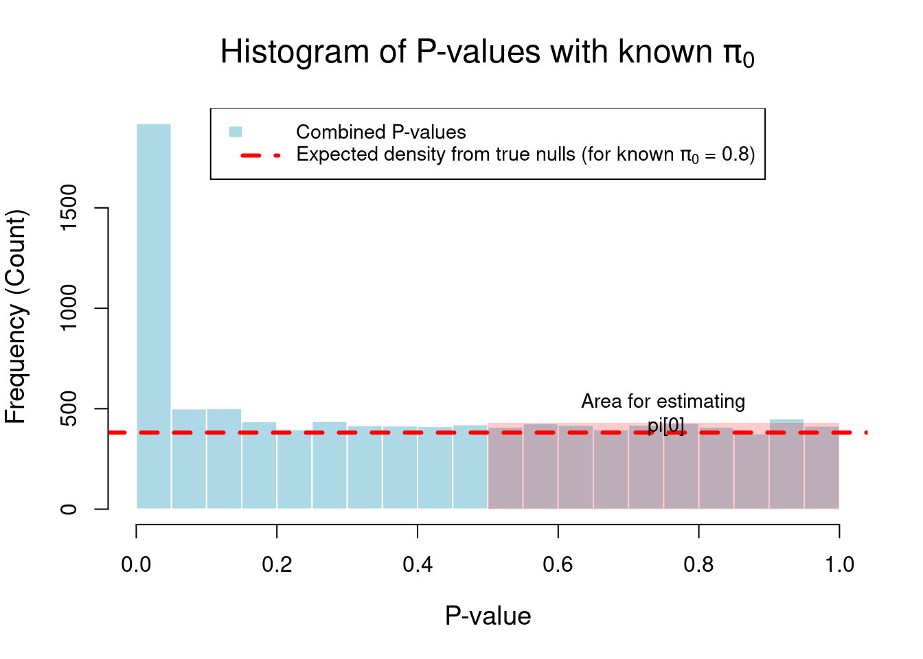
The following R code will simulate a set of p-values where we know the true \(\pi_0\) and then generate a plot that visually demonstrates the logic.
Code
# 1. Simulation Setupset.seed(42) # for reproducibilitym <-10000# Total number of hypothesis testspi0_true <-0.80# We will assume 80% of the null hypotheses are true# Calculate the number of true nulls and true alternativesm0 <- m * pi0_true # Number of true nullsm1 <- m * (1- pi0_true) # Number of true alternatives# 2. Generate P-values# P-values for true nulls follow a uniform distributionp_values_null <-runif(n = m0, min =0, max =1)# P-values for true alternatives are skewed towards 0.# A Beta distribution with shape1 < 1 is a good way to simulate this.p_values_alt <-rbeta(n = m1, shape1 =0.1, shape2 =1)# Combine into a single vector of p-valuesp_values <-sample(c(p_values_null, p_values_alt))# 3. Visualize the Distribution# Plot a histogram of all p-valueshist_info <-hist(p_values, breaks =30, col ="lightblue", border ="white",xlab ="P-value", ylab ="Frequency (Count)",main =expression(paste("Histogram of P-values with known ", pi[0])),cex.main =1.5, cex.lab =1.2)# Add a line representing the expected density of true nulls# The height is the total number of true nulls divided by the number of binsexpected_null_height <- m * pi0_true /length(hist_info$breaks)abline(h = expected_null_height, col ="red", lwd =3, lty =2)# 4. Illustrate the Estimation Logiclambda <-0.5# Choose a tuning parameter lambda# Highlight the area used for estimation (p > lambda)# The y-coordinate is set just above the red line for visibilityrect(xleft = lambda, ybottom =0, xright =1, ytop = expected_null_height +50,col =rgb(1, 0, 0, 0.2), border =NA)text(x = (1+ lambda)/2, y = expected_null_height +100,labels =paste("Area for estimating\n", expression(pi[0])), cex =0.9)legend("top", legend =c("Combined P-values",expression(paste("Expected density from true nulls (for known ", pi[0], " = 0.8)")) ),fill =c("lightblue", NA),border =c("white", NA),lty =c(NA, 2),lwd =c(NA, 3),col =c(NA, "red"),bg ="white",cex =0.9)
Code
# 5. Calculate and Compare# Now, let's use the formula to estimate pi0 from our simulated datanum_p_greater_lambda <-sum(p_values > lambda)pi0_estimate <- num_p_greater_lambda / (m * (1- lambda))# Print the resultscat(paste("True pi0:", pi0_true, "\n"))
True pi0: 0.8
Code
cat(paste("Our estimate of pi0 using lambda =", lambda, "is:", round(pi0_estimate, 4), "\n"))
Our estimate of pi0 using lambda = 0.5 is: 0.8288
Code
# For comparison, let's see what the qvalue package estimateslibrary(qvalue)pi0_qvalue_pkg <-qvalue(p = p_values)$pi0cat(paste("The qvalue package estimates pi0 as:", round(pi0_qvalue_pkg, 4), "\n"))
The qvalue package estimates pi0 as: 0.8368
There is a sharp spike for p-values near 0. This is the contribution from the 2,000 true alternatives.
For p-values greater than ~0.2, the distribution flattens out.
The dashed red line shows the theoretical average height we would expect from the 8,000 true null p-values. You can see that the flat part of the histogram hovers right around this line, visually confirming our assumption.
The transparent red box highlights the region (\(p > 0.5\)) that the formula uses. The logic is that the average height of the histogram bars in this box, when properly scaled, gives an estimate of \(\pi_0\).
The printed output will show that our simple calculation using \(\lambda=0.5\) gives an estimate of \(\pi_0\) that is very close to the true value of 0.8, as does the more sophisticated estimate from the qvalue package. This demonstrates that the logic of using the flat part of the p-value distribution is a sound and effective method for estimating the proportion of true null hypotheses.
2. Calculating the False Discovery Rate (FDR) for a given p-value threshold (\(t\)): With an estimate of \(\pi_0\), the FDR (the expected proportion of false positives among all the rejected hypotheses) for a given p-value threshold \(t\) can be estimated as:
\(\hat{FDR}(t) = \frac{\hat{\pi}_0 \cdot m \cdot t}{\#\{p_i \le t\}}\)
where:
\(\hat{\pi}_0\) is the estimated proportion of true null hypotheses.
\(m\) is the total number of tests.
\(t\) is the p-value threshold.
\(\#\{p_i \le t\}\) is the number of p-values less than or equal to the threshold \(t\).
This formula for the estimated False Discovery Rate (FDR) is best understood as a simple ratio:
\(\hat{FDR}(t) = \frac{\text{Estimated \# of False Positives}}{\text{Observed \# of Total Discoveries}}\)
The denominator, \(\#\{p_i \le t\}\) is the Observed Number of Total Discoveries. It’s a direct count. If you set your p-value cutoff to \(t\) (e.g., 0.05), you simply count how many of your tests have a p-value at or below that threshold. This is the total number of “discoveries” you have made.
The numerator, \(\hat{\pi}_0 \cdot m \cdot t\) is the Estimated Number of False Positives. A false positive can only happen when the null hypothesis is actually true. The logic follows in two steps:
How many true null tests are there? We have \(m\) total tests. We estimate that a proportion \(\hat{\pi}_0\) of them are true nulls. So, our best guess for the total number of true null tests is \(\hat{\pi}_0 \cdot m\).
How many of them will look significant by chance? For a true null test, the p-values are uniformly distributed between 0 and 1. This means the probability of a p-value being less than or equal to \(t\) is simply \(t\).
Combining these, the expected number of false positives is (The number of true null tests) \(\times\) (The probability of any one of them having \(p \le t\)), which gives us \((\hat{\pi}_0 \cdot m) \times t\).
So, the formula:
\(\hat{FDR}(t) = \frac{\hat{\pi}_0 \cdot m \cdot t}{\#\{p_i \le t\}}\)
simply divides the expected number of things that are significant by chance (false positives) by the total number of things we observed to be significant (all discoveries). The result is the estimated proportion of our discoveries that are false.
Quick example: You run 1,000 tests (\(m=1000\)) and you estimate that 80% of them are true nulls (\(\hat{\pi}_0=0.8\)). You set a p-value cutoff of 0.05 (\(t=0.05\)) and find that 70 tests are significant (\(\#\{p_i \le 0.05\}=70\)).
The intuition is: “We made 70 discoveries. We expect 40 of those to be flukes from the true nulls. Therefore, we estimate that about 57% of our discoveries are false.”
3. Calculating the q-value for each p-value: The q-value for a specific p-value \(p_i\) is the minimum estimated FDR that can be achieved when calling all tests with p-values less than or equal to \(p_i\) significant. To ensure monotonicity (q-values should increase as p-values increase), the q-value of the i-th ordered p-value \(p_{(i)}\) is the estimated FDR of \(p_{(i)}\) but is also adjusted to be no smaller than the q-value of the (i-1)-th ordered p-value.
This step ensures that the q-values are well-behaved and can be used as a significance measure. Let me be clearer about what this means exactly: imagine we’ve already calculated our p-values and estimated \(\hat{\pi}_0\). Our goal now is to give each individual test a score that represents the False Discovery Rate. This score is the q-value.
An intuitive first attempt might be: “For each p-value, let’s just calculate the FDR as if that p-value were our cutoff.” Let’s call this the “Pointwise FDR”.
Pointwise FDR at \(p_i\) = \(\frac{\hat{\pi}_0 \cdot m \cdot p_i}{\text{Number of p-values } \le p_i}\)
Let’s see what can happen when we do this. Suppose we have 10,000 tests (\(m=10000\)) and we’ve estimated that \(\hat{\pi}_0 = 0.9\). Let’s look at our top 5 most significant (ordered) p-values:
Rank (i)
p-value \(p_{(i)}\)
# of p-values \(\le p_{(i)}\)
Pointwise FDR (Numerator / Denominator)
Result
1
0.0001
1
(0.9 * 10000 * 0.0001) / 1
0.90
2
0.0003
2
(0.9 * 10000 * 0.0003) / 2
1.35
3
0.0004
3
(0.9 * 10000 * 0.0004) / 3
1.20
4
0.0010
4
(0.9 * 10000 * 0.0010) / 4
2.25
5
0.0011
5
(0.9 * 10000 * 0.0011) / 5
1.98
Look at the results for ranks 4 and 5. The p-value for rank 4 (0.0010) is more significant than the p-value for rank 5 (0.0011). However, it has a higher estimated FDR (2.25 vs 1.98)!
This makes no sense. As we consider less and less significant results, our error rate should not suddenly go down. This property is called non-monotonicity, and it makes the “Pointwise FDR” a poor and uninterpretable measure for individual tests. A significance measure should always be ordered—more significant tests should have a better (lower) score.
This is where the solution of the q-value comes from. It fixes the “bumpiness” by enforcing a simple, logical rule:
The q-value of a test can never be better (lower) than the q-value of a more significant test.
To achieve this, we calculate the q-value for a given p-value, \(p_{(i)}\), by looking at its own Pointwise FDR and the Pointwise FDR of all the tests that are less significant than it. We then assign it the minimum value in that set.
In words: “To find the q-value for the i-th test, look at the Pointwise FDR for the i-th test, the (i+1)-th test, the (i+2)-th test, and so on, all the way to the end. Take the smallest value you find. That’s your q-value.”
Let’s re-calculate our table, but this time we’ll calculate the q-value. The easiest way to do this is to start from the least significant p-value and work backwards.
Let’s add a few more p-values to our list for a better example.
Rank (i)
p-value \(p_{(i)}\)
Pointwise FDR
Calculation of q-value (working backwards)
Final q-value
1
0.0001
0.90
min(0.90, q-value of rank 2) = min(0.90, 1.20)
0.90
2
0.0003
1.35
min(1.35, q-value of rank 3) = min(1.35, 1.20)
1.20
3
0.0004
1.20
min(1.20, q-value of rank 4) = min(1.20, 1.98)
1.20
4
0.0010
2.25
min(2.25, q-value of rank 5) = min(2.25, 1.98)
1.98
5
0.0011
1.98
min(1.98, q-value of rank 6) = min(1.98, 2.05)
1.98
6
0.0015
2.05
min(2.05, q-value of rank 7) = min(2.05, 2.10)
2.05
7
0.0018
2.10
min(2.10, q-value of rank 8) = … (assume it’s higher)
2.10
…
…
…
… (this process continues)
…
The final q-value column is now monotonic: the values only increase as the p-values increase. This makes the q-value an interpretable and reliable measure of significance.
Summary of Intuition
We start by calculating a “raw” or “Pointwise” FDR for every p-value threshold.
We notice this raw measure is bumpy and illogical—a more significant p-value can have a worse FDR than a less significant one.
To fix this, we enforce monotonicity. The q-value for any given test is defined as the most optimistic (lowest) possible FDR you can get by setting your significance cutoff at this test’s p-value or any less significant p-value.
This ensures that as you move down your list of significant results, your expected proportion of false positives (your FDR) can only go up, which is exactly the behavior you’d expect.
Bonferroni Correction vs. Storey’s Method: A Contrast
Feature
Bonferroni Correction
Storey’s Method (q-values)
Error Rate Controlled
Family-Wise Error Rate (FWER)
False Discovery Rate (FDR)
Definition of Error Rate
The probability of making at least one Type I error.
The expected proportion of false positives among rejected hypotheses.
Conservativeness
Generally more conservative, leading to lower statistical power.
Generally less conservative, leading to higher statistical power.
Assumption about True Nulls
Implicitly assumes all null hypotheses could be true (i.e., \(\pi_0=1\)).
Estimates the proportion of true null hypotheses (\(\pi_0\)) from the data.
Best Use Case
When any single false positive is highly problematic (e.g., clinical trials).
When a certain proportion of false positives is acceptable to gain more discoveries (e.g., exploratory genomics research).
Implementation in R
Both the Bonferroni correction and Storey’s method for q-values can be readily implemented in R.
To calculate q-values using Storey’s method, you will need to install and load the qvalue package from Bioconductor.
# Install the qvalue package by install_github("jdstorey/qvalue")# Load the qvalue librarylibrary(qvalue)# Use the same vector of p-valuesset.seed(123)p_values <-c(runif(10, 0, 0.05), runif(90, 0, 1))# Calculate q-valuesq_obj <-qvalue(p = p_values)# View the q-valuesq_values <- q_obj$qvalues# View the original p-values and their corresponding q-valuesdata.frame(Original_P_Value = p_values,Q_Value = q_values)
# Find significant results at an FDR of 0.05significant_qvalues <- q_values <0.05sum(significant_qvalues)
[1] 0
# The qvalue object also contains an estimate of pi0q_obj$pi0
[1] 0.813365
The qvalue object provides not only the q-values but also the estimated proportion of true null hypotheses (\(\pi_0\)). This can be a valuable piece of information for understanding the overall landscape of the hypothesis tests.
Conclusion
In summary, both the Bonferroni correction and Storey’s method of q-values are essential tools for managing the challenges of multiple hypothesis testing. The choice between them depends on the specific goals of the analysis and the tolerance for different types of errors. The Bonferroni method offers stringent control over making even a single false discovery, while Storey’s method provides a more powerful approach for discovery-oriented research where a controlled proportion of false positives is acceptable. The implementation in R allows researchers and students to apply these robust statistical methods to their own data.