Singular value decomposition
Introduction
Many economic datasets can be represented by a rectangular matrix. Let \(X\) contain \(N\) observations in its rows and \(k\) variables in its columns. A row might describe a worker, firm, municipality, or country. A column might record income, schooling, productivity, or employment. Even when \(k\) is large, much of the variation often moves along a smaller number of directions. Income, schooling, and productivity, for example, may share a common direction associated with economic development.
The singular value decomposition, or SVD, identifies these directions. For any real \(m\times n\) matrix \(A\), it produces three matrices such that
\[ A=U\Sigma V^\top. \]
The formula is compact, but it does not by itself convey what the three factors mean. The columns of \(V\) identify orthogonal directions among the inputs. The diagonal entries of \(\Sigma\) state how strongly \(A\) acts along each direction. The columns of \(U\) identify the corresponding directions among the outputs. Thus, the SVD describes a matrix by matching input directions to output directions and attaching a scale to every match.
The discussion below begins with a two-dimensional transformation because its geometry can be drawn. It then establishes the decomposition for every real rectangular matrix and applies it to a synthetic dataset with 160 observations and 4 economic variables. The final sections connect the same decomposition to principal components, low-rank approximation, least squares, and multicollinearity.
A matrix turns a circle into an ellipse
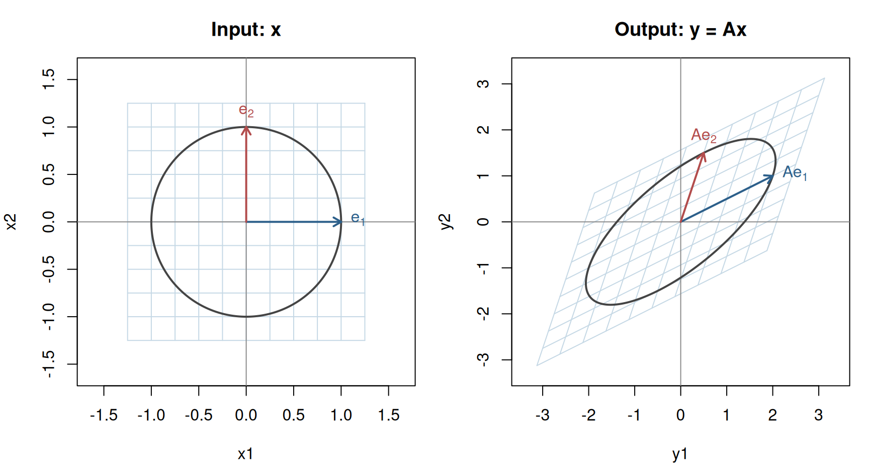
A matrix represents a linear transformation. In two dimensions, its action can be seen by applying it to a square grid and to the unit circle. The matrix used in Figure 1 is
\[ A= \begin{pmatrix} 2 & 0.5\\ 1 & 1.5 \end{pmatrix}, \qquad x=\begin{pmatrix}x_1\\x_2\end{pmatrix} \quad\Longrightarrow\quad y=Ax=\begin{pmatrix}2x_1+0.5x_2\\x_1+1.5x_2\end{pmatrix}. \]
Here \(x_1,x_2\) are coordinates in the standard input basis \(e_1=(1,0)^\top\), \(e_2=(0,1)^\top\), and \(y_1,y_2\) are coordinates in the standard output basis. The columns of \(A\) give \(Ae_1=(2,1)^\top\) and \(Ae_2=(0.5,1.5)^\top\). Thus, moving one unit horizontally in the input moves the output two units horizontally and one vertically. Moving one unit vertically in the input moves the output half a unit horizontally and one and a half vertically. Every other image follows by addition: \(Ax=x_1Ae_1+x_2Ae_2\).
Linearity rules out bending of grid lines: \(A(x+y)=Ax+Ay\) and \(A(cx)=cAx\). The image of the unit circle is an ellipse centered at the origin, as the parameterization in the figure notes shows. If a matrix collapses one direction, the ellipse becomes a line segment or a point. In higher dimensions, the unit sphere becomes an ellipsoid, possibly degenerate, inside the column space of \(A\).
An ellipse has perpendicular principal axes. For this transformation, there are also perpendicular unit input directions whose images lie along those axes. The existence proof below establishes this by choosing eigenvectors of \(A^\top A\). Denote the input directions by \(v_1\) and \(v_2\), their unit output directions by \(u_1\) and \(u_2\), and the corresponding output lengths by \(\sigma_1\) and \(\sigma_2\). They satisfy
\[ Av_1=\sigma_1u_1, \qquad Av_2=\sigma_2u_2. \]
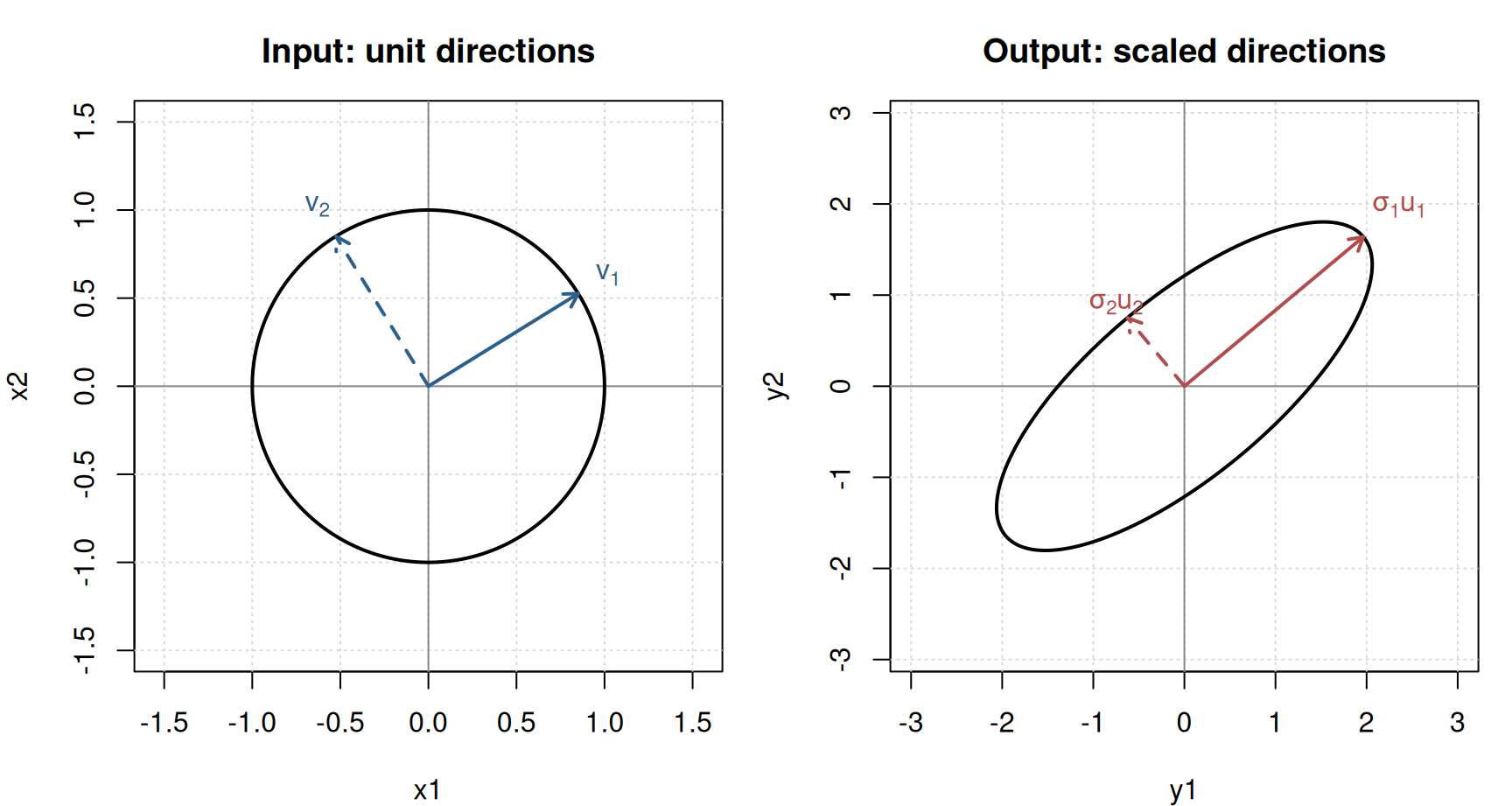
The directions \(v_j\) are the right singular vectors, the directions \(u_j\) are the left singular vectors, and the nonnegative numbers \(\sigma_j\) are the singular values. Singular values are conventionally ordered from largest to smallest. The first pair therefore describes the direction that \(A\) stretches most strongly.
Three simple operations
The factorization \(A=U\Sigma V^\top\) is read from right to left. To interpret the factors, distinguish the vector from the numbers used to describe it. Initially, \(x=(x_1,x_2)^\top\) gives its standard coordinates, meaning \(x=x_1e_1+x_2e_2\). The same vector can also be written in the orthonormal basis formed by the columns of \(V=[v_1\ v_2]\):
\[ x=c_1v_1+c_2v_2=Vc. \]
Multiplying this equation by \(v_i^\top\) gives \(v_i^\top x=c_i\), because \(v_i^\top v_i=1\) and \(v_i^\top v_j=0\) for \(i\ne j\).1 Collecting these two dot products therefore gives
\[ c=V^\top x= \begin{pmatrix}v_1^\top x\\v_2^\top x\end{pmatrix}, \qquad V^\top V=I. \]
Thus \(V^\top\) converts standard input coordinates into coordinates in the \(v\) basis. Each \(c_j\) is a signed scalar projection. The projected vector in the original input space is \(c_jv_j=v_jv_j^\top x\). Keeping both coordinates retains the entire vector, since \(v_1v_1^\top x+v_2v_2^\top x=x\). Keeping only one projected vector would discard its perpendicular component.
Why does scaling these input coordinates give coordinates in the \(u\) basis? The reason is the way the two bases are paired: \(Av_j=\sigma_ju_j\). Apply \(A\) to the expansion of \(x\), using linearity:
\[ \begin{aligned} x&=c_1v_1+c_2v_2,\\ Ax&=c_1Av_1+c_2Av_2\\ &=c_1\sigma_1u_1+c_2\sigma_2u_2. \end{aligned} \]
The last line already expresses the output as a combination of \(u_1\) and \(u_2\). Its coefficient on \(u_1\) is therefore \(b_1=\sigma_1c_1\), and its coefficient on \(u_2\) is \(b_2=\sigma_2c_2\). An input contribution \(c_jv_j\) produces an output contribution \(c_j\sigma_ju_j\): the coefficient is scaled, and the direction changes according to the action of \(A\). Collecting those output coefficients gives
\[ \underbrace{\begin{pmatrix}b_1\\b_2\end{pmatrix}}_{\text{coordinates of }Ax\text{ in the }u\text{ basis}} = \underbrace{\begin{pmatrix}\sigma_1&0\\0&\sigma_2\end{pmatrix}}_{\Sigma} \underbrace{\begin{pmatrix}c_1\\c_2\end{pmatrix}}_{\text{coordinates of }x\text{ in the }v\text{ basis}}. \]
Thus, \(\Sigma\) represents the transformation \(A\) with inputs expressed in the \(v\) basis and outputs expressed in the \(u\) basis. Its column \(j\) contains the \(u\) coordinates of \(Av_j\). Only coordinate \(j\) is nonzero, because \(Av_j\) lies entirely along \(u_j\); this is why the matrix is diagonal. The different meanings of the input and output coordinates are part of this representation. Multiplying by a diagonal matrix in a single fixed basis would simply scale components in that same basis.
This interpretation can also be checked directly by extracting the output coordinates. The last step uses that \(u_1\) and \(u_2\) are orthonormal as well, so that \(u_i^\top u_j\) equals one when \(i=j\) and zero otherwise:2
\[ b_i=u_i^\top Ax =\sum_{j=1}^2c_j u_i^\top Av_j =\sum_{j=1}^2c_j\sigma_j u_i^\top u_j =\sigma_i c_i. \]
Equivalently, \(U^\top AV=\Sigma\): \(V\) builds an input from its \(v\) coordinates, \(A\) transforms it, and \(U^\top\) reads the result in \(u\) coordinates. The diagonal matrix carries out this entire mapping between coordinate descriptions. Multiplication by \(U=[u_1\ u_2]\) then converts \(b=\Sigma c\) to standard output coordinates by taking a weighted sum of its columns:
\[ y=Ub=b_1u_1+b_2u_2 =\sigma_1(v_1^\top x)u_1+\sigma_2(v_2^\top x)u_2=Ax. \]
In particular, \(U\) maps the coordinate vector \((1,0)^\top\) to \(u_1\) and \((0,1)^\top\) to \(u_2\). Its inverse \(U^\top\) extracts the coordinates \(b_j=u_j^\top y\), just as \(V^\top\) does on the input side. The complete sequence is
\[ \begin{aligned} c&=V^\top x &&\text{(standard input coordinates to the }v\text{ basis)},\\ b&=\Sigma c &&\text{(scale to output coordinates in the }u\text{ basis)},\\ y&=Ub=Ax &&\text{(the }u\text{ basis to standard output coordinates)}. \end{aligned} \]
For the matrix \(A\) above, the factors are approximately
\[ V=\begin{pmatrix}0.851&-0.526\\0.526&0.851\end{pmatrix}, \quad \Sigma=\begin{pmatrix}2.558&0\\0&0.977\end{pmatrix}, \quad U=\begin{pmatrix}0.768&-0.641\\0.641&0.768\end{pmatrix}. \]
Take \(x=(1,0)^\top\), the green arrow in the first panel of Figure 3. Its coordinates in the \(v\) basis are
\[ c=V^\top x\approx\begin{pmatrix}0.851\\-0.526\end{pmatrix}, \qquad x\approx0.851v_1-0.526v_2. \]
The second coordinate is negative because \(x\) points partly opposite to \(v_2\). After scaling,
\[ b=\Sigma c\approx\begin{pmatrix}2.176\\-0.514\end{pmatrix}. \]
In terms of vectors, the first input contribution \(0.851v_1\) is sent to \(0.851Av_1=0.851\sigma_1u_1\approx2.176u_1\). The second contribution \(-0.526v_2\) is sent to \(-0.526Av_2=-0.526\sigma_2u_2\approx-0.514u_2\). This is why the numbers \(2.176\) and \(-0.514\) multiply \(u_1\) and \(u_2\) in the output. Panels 2 and 3 of Figure 3 plot these input and output coefficients, respectively.
Finally, the output in standard coordinates is
\[ y=Ub\approx 2.176\begin{pmatrix}0.768\\0.641\end{pmatrix} -0.514\begin{pmatrix}-0.641\\0.768\end{pmatrix} \approx\begin{pmatrix}2\\1\end{pmatrix} =A\begin{pmatrix}1\\0\end{pmatrix}. \]
All displayed factors and intermediate coordinates are rounded; the unrounded product is exactly \((2,1)^\top\).
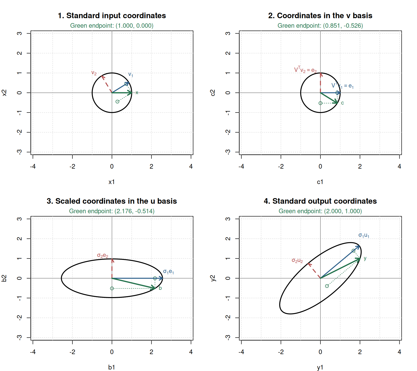
When a coordinate tuple is plotted in a new panel, \(V^\top\) makes the picture appear rotated or reflected. As a change of basis, this describes the same input vector with different coordinates. Similarly, \(U\) expresses the output coordinates \(b\) in the standard basis. Orthogonal matrices such as \(V^\top\) and \(U\) preserve lengths and angles.3 All changes in length occur inside \(\Sigma\). This separation explains why singular values measure the strength of a transformation. A direction associated with a small singular value has little effect on the output, whereas a direction associated with a zero singular value disappears entirely.
For a general \(m\times n\) matrix, the full decomposition has the following dimensions.
| Object | Dimensions | Interpretation |
|---|---|---|
| \(V^\top\) | \(n\times n\) | Converts standard input coordinates to the \(v\) basis: \(c_j=v_j^\top x\) |
| \(\Sigma\) | \(m\times n\) | Scales matched coordinates; discards or supplies zero coordinates as needed |
| \(U\) | \(m\times m\) | Converts output coordinates in the \(u\) basis to standard coordinates: \(y=\sum_{j=1}^m b_ju_j\) |
If \(r=\operatorname{rank}(A)\), only \(r\) singular values are positive. The thin SVD, used here to mean the form retaining only these \(r\) directions, is
\[ A=U_rD_rV_r^\top, \]
where \(U_r\) is \(m\times r\), \(D_r\) is \(r\times r\), and \(V_r\) is \(n\times r\). This form contains the same information as the full decomposition without carrying bases for directions that contribute nothing to \(A\). Here \(V_r^\top x\) retains only the coordinates that affect \(Ax\), and \(V_rV_r^\top x\) is the orthogonal projection onto their span. Unlike the full square \(V^\top\), \(V_r^\top\) can therefore discard a component of \(x\) in the null space of \(A\).
A matrix as a sum of layers
Matrix multiplication can also be read one singular direction at a time. Expanding the thin SVD gives
\[ A=\sigma_1u_1v_1^\top+\sigma_2u_2v_2^\top+\cdots+\sigma_ru_rv_r^\top. \]
Each outer product \(u_jv_j^\top\) is a rank-one matrix. Given an input \(x\), the scalar \(v_j^\top x\) is its signed coordinate along \(v_j\). The layer multiplies this coordinate by \(\sigma_j\) and places it along \(u_j\):
\[ \left(\sigma_ju_jv_j^\top\right)x =\sigma_j\left(v_j^\top x\right)u_j. \]
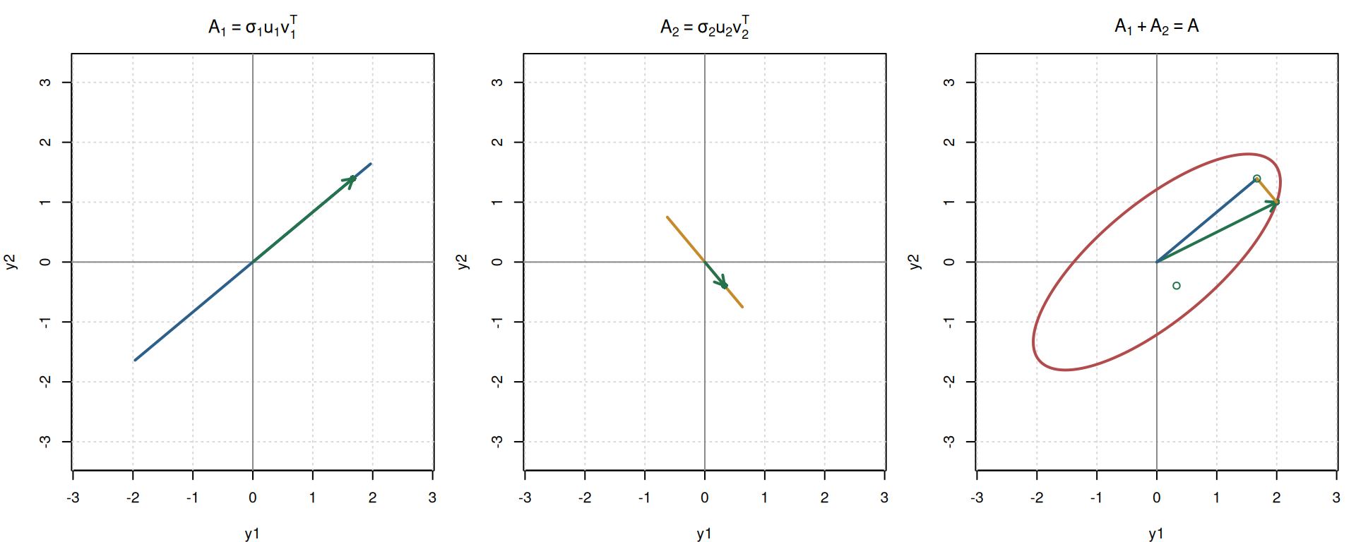
To see precisely how the two layers in Figure 4 produce the ellipse, parameterize the unit circle in the orthonormal input basis:
\[ x(t)=\cos(t)v_1+\sin(t)v_2,\qquad 0\leq t<2\pi. \]
This traces the same unit circle as before, with the angle now measured from \(v_1\). Write \(A_j=\sigma_ju_jv_j^\top\). Orthogonality gives
\[ A_1x(t)=\sigma_1\cos(t)u_1, \qquad A_2x(t)=\sigma_2\sin(t)u_2. \]
Separately, these trace the line segments \([-\sigma_1u_1,\sigma_1u_1]\) and \([-\sigma_2u_2,\sigma_2u_2]\). Matrix addition adds the two outputs for the same input \(x(t)\):
\[ y(t)=(A_1+A_2)x(t) =\sigma_1\cos(t)u_1+\sigma_2\sin(t)u_2. \]
In output coordinates along the \(u\) basis, \(z_j=u_j^\top y\), this gives \(z_1=\sigma_1\cos(t)\) and \(z_2=\sigma_2\sin(t)\), hence
\[ \left(\frac{z_1}{\sigma_1}\right)^2+ \left(\frac{z_2}{\sigma_2}\right)^2=1. \]
This is the ellipse equation with semiaxis lengths \(\sigma_1,\sigma_2\). Conversely, each point satisfying this equation corresponds to a pair \((\cos t,\sin t)\), so the sum traces the entire ellipse. The common input imposes the constraint \(\cos^2t+\sin^2t=1\). Choosing points independently from the two segments would instead fill a rectangle, since their two coefficients could then vary independently in \([-1,1]\).
For the same numerical input \(x=(1,0)^\top\), the contributions are approximately
\[ A_1x=2.176u_1\approx\begin{pmatrix}1.671\\1.394\end{pmatrix}, \qquad A_2x=-0.514u_2\approx\begin{pmatrix}0.329\\-0.394\end{pmatrix}. \]
Their sum is \(Ax=(2,1)^\top\), the green point in the final panel.
This representation also gives the rank of \(A\): it is the number of positive singular values. The right singular vectors associated with positive singular values span the row space, while the remaining right singular vectors span the null space. The left singular vectors associated with positive singular values span the column space.
Why the decomposition exists for every real matrix
The geometric argument identifies the result in two dimensions, but it does not establish the decomposition in higher dimensions. A general proof follows from the spectral theorem for real symmetric matrices: if \(B=B^\top\), then \(B\) has an orthonormal basis of real eigenvectors and all its eigenvalues are real.
Let \(A\in\mathbb R^{m\times n}\) and consider \(A^\top A\). This is a real symmetric matrix because
\[ (A^\top A)^\top=A^\top A. \]
It is also positive semidefinite. For every \(x\in\mathbb R^n\),
\[ x^\top A^\top Ax=\lVert Ax\rVert^2\geq 0. \]
This identity also explains the geometric role of \(A^\top A\): its quadratic form measures the squared length of the output for each input. Every point on the image of the unit sphere is \(Ax\) for some unit vector \(x\). Finding a point farthest from the origin therefore means solving
\[ \max_{\lVert x\rVert=1}\lVert Ax\rVert^2 =\max_{\lVert x\rVert=1}x^\top A^\top Ax. \]
To obtain the right singular vectors, compute the eigenvectors of \(A^\top A\) and choose an orthonormal basis within each eigenspace. The spectral theorem guarantees that this gives \(n\) vectors \(v_1,\ldots,v_n\) with nonnegative eigenvalues \(\lambda_1\geq\cdots\geq\lambda_n\geq0\) satisfying
\[ A^\top Av_j=\lambda_jv_j. \]
To see why these eigenvectors solve the stretching problem, expand a unit input in this orthonormal basis:
\[ x=\sum_{j=1}^n c_jv_j, \qquad \sum_{j=1}^n c_j^2=1. \]
Using the eigenvector equations and orthonormality gives
\[ \lVert Ax\rVert^2 =\sum_{i=1}^n\sum_{j=1}^n c_ic_jv_i^\top A^\top Av_j =\sum_{j=1}^n\lambda_jc_j^2. \]
The coefficients are not fixed: as \(x\) ranges over the unit sphere, the numbers \(c_j^2\) can redistribute one unit of weight across the eigenvalues. Since \(\lambda_j\leq\lambda_1\) for every \(j\),
\[ \lVert Ax\rVert^2 =\sum_{j=1}^n\lambda_jc_j^2 \leq\sum_{j=1}^n\lambda_1c_j^2 =\lambda_1. \]
The upper bound is attained by putting all weight on the first eigenvector: \(x=v_1\) or \(x=-v_1\) gives \(c_1^2=1\) and \(c_j=0\) for \(j>1\). Equivalently, no mixture of directions can produce a squared length larger than the largest number being averaged. If the largest eigenvalue is repeated, every unit vector in its eigenspace also attains the maximum; \(\pm v_1\) are particular maximizing directions. The analogous inequality \(\lambda_j\geq\lambda_n\) gives \(\lVert Ax\rVert^2\geq\lambda_n\), with equality at \(\pm v_n\) (and, if the smallest eigenvalue is repeated, throughout its eigenspace).
More generally, among unit inputs perpendicular to \(v_1,\ldots,v_{j-1}\), the first \(j-1\) coefficients vanish. Repeating the same bound over the remaining terms gives a maximum of \(\lambda_j\), attained at \(\pm v_j\); if \(\lambda_j\) is repeated among the remaining eigenvalues, the entire corresponding unit eigensphere attains it. Thus the eigenvectors identify successive directions of greatest stretching subject to orthogonality to the preceding input directions. In particular, the image of \(v_1\) lies on a longest semiaxis of the ellipse, while the image of \(v_n\) lies on a shortest semiaxis.
The eigenvalues measure squared stretch factors. For a unit eigenvector \(v_j\),
\[ \lVert Av_j\rVert^2 =(Av_j)^\top(Av_j) =v_j^\top(A^\top A)v_j =\lambda_j\lVert v_j\rVert^2 =\lambda_j, \qquad \lVert Av_j\rVert=\sqrt{\lambda_j}=\sigma_j. \]
The composition \(A^\top A\) applies \(A\) and then \(A^\top\): along the paired singular directions, each scales by \(\sigma_j\), so the factors multiply to \(\sigma_j^2\). In matrix form, \(A^\top A=V\Sigma^\top\Sigma V^\top\) (or \(V\Sigma^2V^\top\) when \(\Sigma\) is square). Using \(\lambda_j\) as the stretch factor would therefore apply the scaling twice; taking its square root gives the stretch under \(A\) alone.
Conventionally, a rectangular matrix has \(\min(m,n)\) listed singular values; if \(n>m\), the remaining \(n-m\) eigenvalues of \(A^\top A\) are necessarily zero. To obtain the corresponding left singular vector when \(\sigma_j>0\), multiply \(v_j\) by \(A\) and divide by its length:
\[ u_j=\frac{Av_j}{\sigma_j}. \]
This formula specifies the pairing: \(v_j\) is an input direction, \(Av_j\) is its image, \(\sigma_j=\lVert Av_j\rVert\) is the amount of stretching, and \(u_j\) is the unit direction of that image. This equality follows because \(v_j\) has unit length and \(\lVert Av_j\rVert^2=v_j^\top A^\top Av_j=\lambda_j=\sigma_j^2\); both quantities are nonnegative. Geometrically, \(Av_j\) is the endpoint in the output space obtained by applying \(A\) to the unit arrow \(v_j\). In particular, \(Av_1\) points toward the farthest stretch of the unit circle, because \(v_1\) maximizes \(\lVert Ax\rVert\) over unit input vectors. The vectors \(u_j\) are also eigenvectors of \(AA^\top\), since
\[ AA^\top u_j =\frac{A(A^\top Av_j)}{\sigma_j} =\frac{A(\lambda_jv_j)}{\sigma_j} =\lambda_ju_j =\sigma_j^2u_j. \]
Thus, \(A^\top A\) determines directions in the \(n\)-dimensional input space, whereas \(AA^\top\) determines directions in the \(m\)-dimensional output space. Their positive eigenvalues coincide. One could start with the eigenvectors of \(AA^\top\) instead and recover \(v_j=A^\top u_j/\sigma_j\). Constructing one set from the other ensures that their signs and, for repeated eigenvalues, their chosen bases are paired consistently.
The constructed \(u_j\) have unit length and are mutually orthogonal. Indeed,
\[ u_i^\top u_j =\frac{v_i^\top A^\top Av_j}{\sigma_i\sigma_j} =\frac{\lambda_jv_i^\top v_j}{\sigma_i\sigma_j} = \begin{cases} 1,&i=j,\\ 0,&i\neq j. \end{cases} \]
This orthogonality connects the construction to the principal axes. Consider an invertible \(2\times2\) matrix, so that \(\sigma_1\geq\sigma_2>0\). The stretching argument shows that \(Av_1=\sigma_1u_1\) reaches a farthest point on the output ellipse, while \(Av_2=\sigma_2u_2\) reaches a nearest point. Normalizing these images preserves their directions, so \(u_1\) and \(u_2\) point along the major and minor axes. Although \(A\) need not preserve perpendicularity for arbitrary input directions, the calculation above proves that these particular images are perpendicular.
The equation of the entire ellipse makes the connection explicit. Every unit input has the form \(x=c_1v_1+c_2v_2\), with \(c_1^2+c_2^2=1\), because \(v_1\) and \(v_2\) are orthonormal and hence \(\lVert x\rVert^2=c_1^2+c_2^2\). Linearity gives
\[ y=Ax=\sigma_1c_1u_1+\sigma_2c_2u_2. \]
Since \(u_1,u_2\) are orthonormal, the output coordinates along them are \(z_j=u_j^\top y=\sigma_jc_j\). The unit-circle constraint applies to the input coordinates \(c_1,c_2\), not to the output coordinates \(z_1,z_2\): the map stretches the \(j\)th coordinate by \(\sigma_j\). Solving the preceding relation \(z_j=\sigma_jc_j\) for \(c_j\) gives \(c_j=z_j/\sigma_j\), which, substituted into the input constraint, yields
\[ \frac{z_1^2}{\sigma_1^2}+\frac{z_2^2}{\sigma_2^2}=1. \]
Thus, after rescaling each output coordinate by its singular value, \((z_1/\sigma_1,z_2/\sigma_2)\) lies on the unit circle. The output vector itself need not have unit length; its coordinates trace an ellipse. Conversely, every pair satisfying this equation gives a unit input by setting \(c_j=z_j/\sigma_j\). This is therefore exactly the image of the circle, expressed in perpendicular coordinates along the constructed \(u\) vectors. Its principal axis directions are \(u_1,u_2\), and its semiaxis lengths are \(\sigma_1,\sigma_2\). If the singular values coincide, the image is a circle and any orthonormal pair in its plane can serve as axes. The freedom to choose eigenvectors within a repeated eigenspace corresponds to this geometric symmetry.
In higher dimensions, the same coordinate argument identifies the positive-singular-value directions \(u_j\) as the axes of the image ellipsoid. To include rank-deficient matrices, consider the image of the unit ball \(\lVert x\rVert\leq1\): it is the filled ellipsoid in the column space of \(A\), with semiaxis lengths given by the positive singular values. Input directions with zero singular values collapse to zero; completing the output basis adds directions perpendicular to that column space.
Let \(r\) be the number of positive singular values, which equals the rank of \(A\). The construction gives an orthonormal basis \(u_1,\ldots,u_r\) for the column space of \(A\). If \(r<m\), complete it to an orthonormal basis of \(\mathbb R^m\) by choosing \(m-r\) unit vectors in its orthogonal complement, the null space of \(A^\top\). These additional vectors satisfy \(A^\top u_j=0\) and hence \(AA^\top u_j=0\): they are eigenvectors for the zero eigenvalue of \(AA^\top\). No division by a zero singular value is required. Place this full basis in the columns of \(U\), place \(v_1,\ldots,v_n\) in the columns of \(V\), and put the \(r\) positive singular values on the diagonal of the \(m\times n\) matrix \(\Sigma\), with zeros elsewhere.
It remains to check the directions with zero singular values. If \(j>r\), then
\[ \lVert Av_j\rVert^2 =v_j^\top A^\top Av_j =\lambda_j =0, \]
so \(Av_j=0\). Consequently, \(A\) and \(U\Sigma V^\top\) agree on every basis vector \(v_j\): both send \(v_j\) to \(\sigma_ju_j\) when \(j\leq r\), and both send it to zero otherwise. Two linear transformations that agree on a basis are equal. Hence
\[ A=U\Sigma V^\top. \]
The dimensions and the completion of the bases can be displayed explicitly. Write \(U_r=[u_1\ \cdots\ u_r]\) for the constructed output directions and \(U_0=[u_{r+1}\ \cdots\ u_m]\) for their orthonormal completion. Similarly, write \(V_r=[v_1\ \cdots\ v_r]\) and \(V_0=[v_{r+1}\ \cdots\ v_n]\). Then the full decomposition is
\[ \underbrace{A}_{m\times n} = \underbrace{\left[\begin{array}{c|c}U_r&U_0\end{array}\right]}_{U:\ m\times m} \underbrace{\left[\begin{array}{c|c} D_r&0\\\hline 0&0 \end{array}\right]}_{\Sigma:\ m\times n} \underbrace{\left[\begin{array}{c} V_r^\top\\\hline V_0^\top \end{array}\right]}_{V^\top:\ n\times n}, \qquad D_r=\begin{pmatrix} \sigma_1&&0\\ &\ddots&\\ 0&&\sigma_r \end{pmatrix}. \]
The partition in \(\Sigma\) occurs after row \(r\) and column \(r\). Its four blocks have dimensions
\[ \Sigma= \begin{pmatrix} (D_r)_{r\times r}&0_{r\times(n-r)}\\ 0_{(m-r)\times r}&0_{(m-r)\times(n-r)} \end{pmatrix}. \]
The columns of \(U\) and the rows of \(V^\top\) are arranged as follows:
\[ U= \left[\begin{array}{ccc|ccc} \vert&&\vert&\vert&&\vert\\ u_1&\cdots&u_r&u_{r+1}&\cdots&u_m\\ \vert&&\vert&\vert&&\vert \end{array}\right], \qquad V^\top= \left[\begin{array}{c} v_1^\top\\\vdots\\v_r^\top\\\hline v_{r+1}^\top\\\vdots\\v_n^\top \end{array}\right]. \]
Here \(U_r\) is \(m\times r\) and \(U_0\) is \(m\times(m-r)\); every column has \(m\) entries. Likewise, \(V_r\) is \(n\times r\) and \(V_0\) is \(n\times(n-r)\). The \(m-r\) added columns of \(U\) are unit vectors perpendicular to the column space of \(A\), chosen to be mutually orthogonal. Their coefficients are always zero in \(Ax\), as the bottom \(m-r\) rows of \(\Sigma\) show. The \(n-r\) columns of \(V_0\) are input directions annihilated by \(A\), as the rightmost \(n-r\) columns of \(\Sigma\) show. Multiplying the blocks leaves \(A=U_rD_rV_r^\top\). If a block has zero rows or columns, it is simply absent; if \(r=0\), then \(A=0\) and both full bases can be chosen freely subject to orthonormality.
For example, a \(4\times3\) matrix of rank \(2\) has the full decomposition
\[ \underbrace{A}_{4\times3} = \underbrace{\left[\begin{array}{cc|cc} u_1&u_2&u_3&u_4 \end{array}\right]}_{U:\ 4\times4} \underbrace{\left[\begin{array}{cc|c} \sigma_1&0&0\\ 0&\sigma_2&0\\\hline 0&0&0\\ 0&0&0 \end{array}\right]}_{\Sigma:\ 4\times3} \underbrace{\left[\begin{array}{c} v_1^\top\\v_2^\top\\\hline v_3^\top \end{array}\right]}_{V^\top:\ 3\times3}. \]
Only \(u_1=Av_1/\sigma_1\) and \(u_2=Av_2/\sigma_2\) are obtained by dividing images by positive singular values. The columns \(u_3,u_4\) complete the output basis, while \(v_3\) spans the input null space. There are two added columns in \(U\) even though only one of the three listed singular values is zero, because the output space has dimension four.
For a data matrix \(X\in\mathbb R^{N\times k}\), the same count is \(N-r\) additional columns in the full \(U\) and \(k-r\) null directions in the full \(V\). Thus \(r<k\) does indicate fewer positive singular values than variable directions. Completion of \(U\) is required whenever \(r<N\), including the full-column-rank case \(r=k<N\). The rank-\(r\) thin SVD omits both sets of additional columns.
The proof uses only real matrices. It covers tall, wide, square, and rank-deficient matrices. The decomposition need not be unique. The signs of a pair \(u_j,v_j\) can be reversed together, and repeated singular values permit different orthonormal bases within the corresponding subspace. The singular values themselves are nevertheless fixed.
Constructing the decomposition for the two-dimensional example
The proof can be carried out numerically for the same matrix used in the preceding figures. Each step has a geometric counterpart: the eigenvectors of \(A^\top A\) identify the unit inputs with extreme output lengths, their images give the semiaxes of the ellipse, and normalization gives the columns of \(U\). Here
\[ A=\begin{pmatrix}2&0.5\\1&1.5\end{pmatrix}, \qquad B=A^\top A =\begin{pmatrix}2&1\\0.5&1.5\end{pmatrix} \begin{pmatrix}2&0.5\\1&1.5\end{pmatrix} =\begin{pmatrix}5&2.5\\2.5&2.5\end{pmatrix}. \]
Finding the input directions and their stretches
For a unit input \(x(\theta)=(\cos\theta,\sin\theta)^\top\), the squared output length is
\[ q(\theta)=x(\theta)^\top Bx(\theta) =5\cos^2\theta+5\cos\theta\sin\theta+2.5\sin^2\theta. \]
The proof locates the extrema of this expression through the eigenvalues of \(B\). They solve
\[ \det(B-\lambda I) =(5-\lambda)(2.5-\lambda)-2.5^2 =\lambda^2-7.5\lambda+6.25=0, \]
so that
\[ \lambda_1=\frac{15+5\sqrt5}{4}\approx6.5451, \qquad \lambda_2=\frac{15-5\sqrt5}{4}\approx0.9549. \]
For each eigenvalue, the first row of \((B-\lambda_jI)v_j=0\) gives \(v_{j,2}/v_{j,1}=(\lambda_j-5)/2.5\). Normalizing these vectors and choosing their signs as in the earlier figures yields
\[ v_1\approx\begin{pmatrix}0.8507\\0.5257\end{pmatrix}, \qquad v_2\approx\begin{pmatrix}-0.5257\\0.8507\end{pmatrix}, \qquad \sigma_1=\sqrt{\lambda_1}\approx2.5583, \quad \sigma_2=\sqrt{\lambda_2}\approx0.9772. \]
The directions have angles approximately \(31.7175^\circ\) and \(121.7175^\circ\) from the horizontal axis. They are perpendicular, and Figure 5 shows that they attain the maximum and minimum squared output lengths. Opposite inputs give opposite outputs of the same length, so the plot covers \(0\leq\theta\leq180^\circ\).
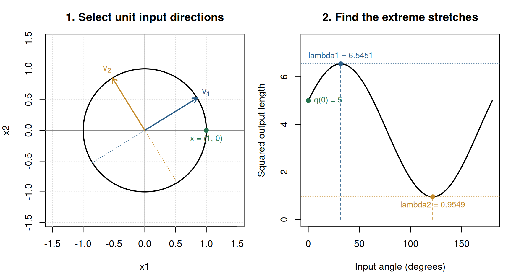
The weighted-average argument in the proof can also be checked with the original input \(x=(1,0)^\top\). Its coefficients are \(c=V^\top x\approx(0.8507,-0.5257)^\top\), so \(c_1^2\approx0.7236\) and \(c_2^2\approx0.2764\). Consequently,
\[ \lVert Ax\rVert^2 =\lambda_1c_1^2+\lambda_2c_2^2 \approx6.5451(0.7236)+0.9549(0.2764) \approx5. \]
Direct multiplication gives \(Ax=(2,1)^\top\), whose squared length is exactly \(5\). This lies between \(0.9549\) and \(6.5451\), as the proof requires.
Constructing the output axes
Multiplying the computed input vectors by \(A\) gives
\[ Av_1\approx\begin{pmatrix}1.9642\\1.6392\end{pmatrix}, \qquad Av_2\approx\begin{pmatrix}-0.6261\\0.7502\end{pmatrix}. \]
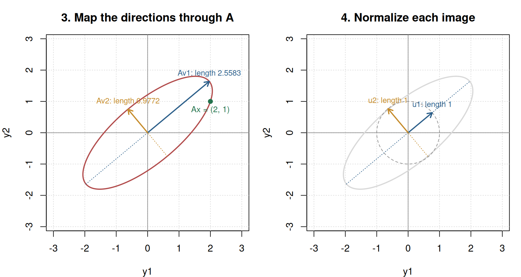
Their lengths are \(2.5583\) and \(0.9772\). Their dot product is zero before rounding: \((Av_1)^\top Av_2=v_1^\top Bv_2=\lambda_2v_1^\top v_2=0\). Thus these images give perpendicular semiaxes, even though the images of the standard basis vectors, \((2,1)^\top\) and \((0.5,1.5)^\top\), have dot product \(2.5\). Dividing each image by its length gives
\[ u_1=\frac{Av_1}{\sigma_1} \approx\frac{1}{2.5583}\begin{pmatrix}1.9642\\1.6392\end{pmatrix} \approx\begin{pmatrix}0.7678\\0.6407\end{pmatrix}, \qquad u_2=\frac{Av_2}{\sigma_2} \approx\frac{1}{0.9772}\begin{pmatrix}-0.6261\\0.7502\end{pmatrix} \approx\begin{pmatrix}-0.6407\\0.7678\end{pmatrix}. \]
In Figure 6, the first panel shows the image vectors on the ellipse, and the second shows their unit directions. Normalization changes their lengths while preserving their perpendicular directions. Both singular values are positive, so both columns of \(U\) are obtained this way and no completion of the basis is needed.
The ellipse equation now follows with actual coefficients. For a point \(y\) in standard output coordinates, its coordinates along the constructed axes are
\[ z_1=u_1^\top y\approx0.7678y_1+0.6407y_2, \qquad z_2=u_2^\top y\approx-0.6407y_1+0.7678y_2. \]
The image of the unit circle therefore satisfies
\[ \frac{z_1^2}{\lambda_1}+\frac{z_2^2}{\lambda_2}=1, \qquad\text{or, approximately,}\qquad \frac{(0.7678y_1+0.6407y_2)^2}{6.5451} +\frac{(-0.6407y_1+0.7678y_2)^2}{0.9549}=1. \]
Using unrounded coefficients and expanding gives \(13y_1^2-22y_1y_2+17y_2^2=25\), the same ellipse obtained earlier by substituting \(x=A^{-1}y\) into the unit-circle equation. At the marked point \(y=(2,1)^\top\), the principal-axis coordinates are \(z\approx(2.1763,-0.5137)^\top\). Dividing by the semiaxis lengths recovers \(c\approx(0.8507,-0.5257)^\top\), whose squared coordinates sum to one.
Computing and checking the factors
Collecting the vectors and lengths gives the numerical factorization
\[ \underbrace{\begin{pmatrix}2&0.5\\1&1.5\end{pmatrix}}_A \approx \underbrace{\begin{pmatrix}0.7678&-0.6407\\0.6407&0.7678\end{pmatrix}}_U \underbrace{\begin{pmatrix}2.5583&0\\0&0.9772\end{pmatrix}}_\Sigma \underbrace{\begin{pmatrix}0.8507&0.5257\\-0.5257&0.8507\end{pmatrix}}_{V^\top}. \]
The following R code implements the construction directly. It computes the eigenvectors of \(A^\top A\), takes square roots of the eigenvalues, and obtains \(U\) by normalizing \(AV\). The sign convention makes the largest absolute entry of each input eigenvector positive, matching the figures. All calculations use unrounded values; only the displayed output is rounded.
A_numeric <- matrix(c(2, 0.5, 1, 1.5), nrow = 2, byrow = TRUE)
e <- eigen(crossprod(A_numeric), symmetric = TRUE)
V_numeric <- e$vectors
for (j in 1:2) {
  pivot <- which.max(abs(V_numeric[, j]))
  if (V_numeric[pivot, j] < 0) V_numeric[, j] <- -V_numeric[, j]
}
Sigma_numeric <- diag(sqrt(e$values))
U_numeric <- A_numeric %*% V_numeric %*% diag(1 / sqrt(e$values))
A_reconstructed <- U_numeric %*% Sigma_numeric %*% t(V_numeric)

lapply(list(U = U_numeric, Sigma = Sigma_numeric,
            V_transpose = t(V_numeric), reconstructed_A = A_reconstructed),
       round, digits = 4)
$U
[,1] [,2]
[1,] 0.7678 -0.6407
[2,] 0.6407 0.7678
$Sigma
[,1] [,2]
[1,] 2.5583 0.0000
[2,] 0.0000 0.9772
$V_transpose
[,1] [,2]
[1,] 0.8507 0.5257
[2,] -0.5257 0.8507
$reconstructed_A
[,1] [,2]
[1,] 2 0.5
[2,] 1 1.5The maximum absolute entrywise reconstruction error is 4.44e-16. Numerical checks also verify orthonormality and agreement with the factors used in the figures. These numerical equalities illustrate the last step of the proof: the reconstructed transformation agrees with \(A\) on both input basis vectors and hence on every input.
The same decomposition for a data table
Consider a data matrix \(X\in\mathbb R^{N\times k}\). The synthetic example contains four variables generated from two latent factors and independent noise. Each column is centered and divided by its sample standard deviation. This standardization prevents a variable from dominating merely because it is recorded in larger units. It also means that the covariance matrix below is the sample correlation matrix of the original variables.
The two-variable view in Figure 7 shows the first connection between the SVD and a dataset. The observations form a point cloud. Its principal directions are the right singular vectors, and its standard deviations along those directions are \(d_j/\sqrt{N-1}\).
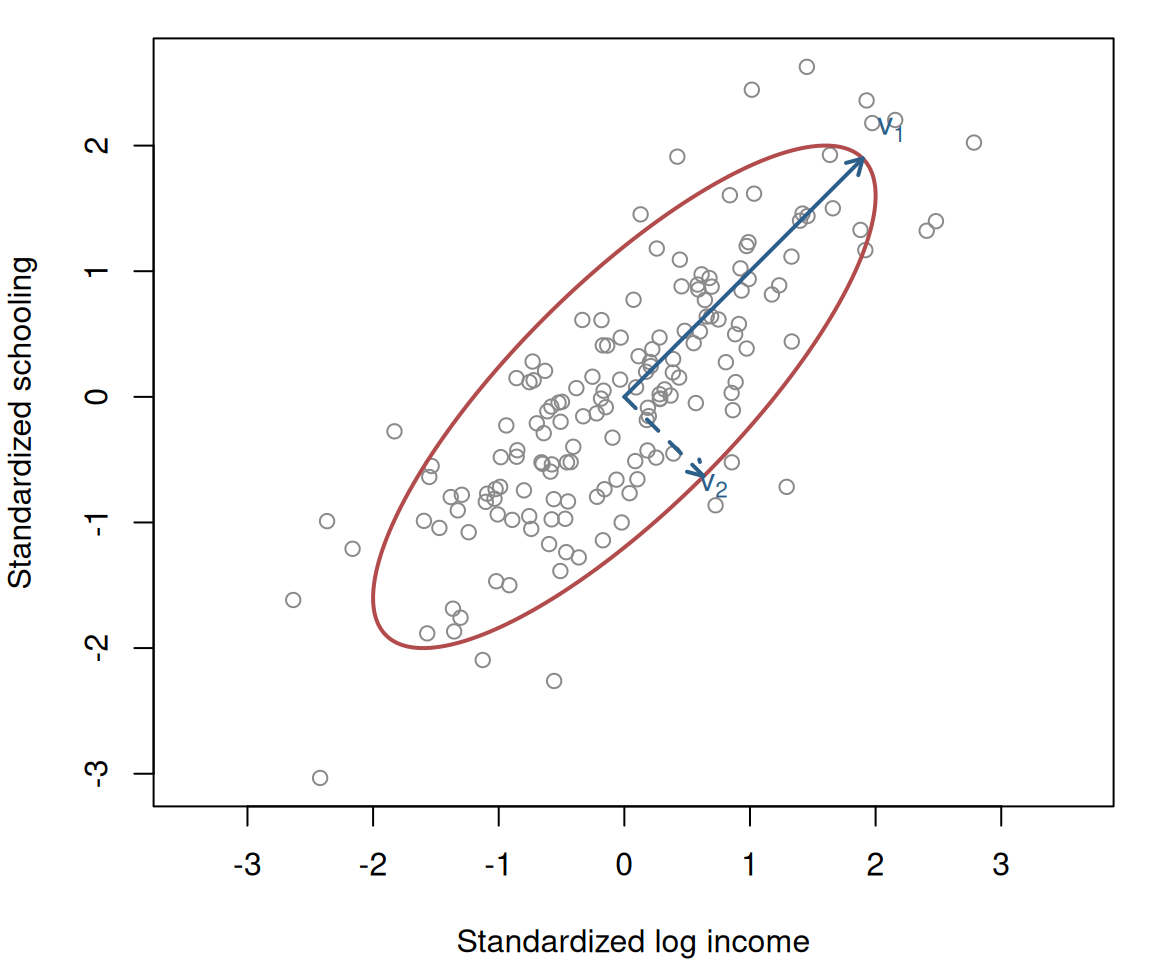
Write the thin SVD of the full data matrix as \(X=UDV^\top\). In this example, all \(k\) columns are linearly independent, so \(U\) has dimensions \(N\times k\), \(D\) has dimensions \(k\times k\), and \(V\) has dimensions \(k\times k\). The notation \(d_j\) denotes the singular values of \(X\), just as \(\sigma_j\) denoted those of \(A\). Its sample covariance matrix is
\[ S=\frac{X^\top X}{N-1} =V\frac{D^2}{N-1}V^\top. \]
The columns of \(V\) are therefore the eigenvectors of the covariance matrix. In principal component terminology, they are the component directions. Some software calls these vectors loadings, whereas other software reserves that term for coefficients scaled by the component standard deviations. The associated covariance eigenvalues are \(d_j^2/(N-1)\). This identity is the algebraic counterpart of the ellipse: \(V\) supplies its axes and \(D/\sqrt{N-1}\) supplies their lengths.
The coordinates of the observations along the new axes are obtained by projecting the rows of \(X\) onto \(V\):
\[ XV=UD. \]
For an individual observation with row \(x_i^\top\), the score on component \(j\) is \(x_i^\top v_j=\sum_{\ell=1}^k x_{i\ell}v_{\ell j}\). Thus, \(UD\) is the matrix of principal-component scores: its \(j\)th column \(d_ju_j=Xv_j\) records the location of every observation along component \(j\). The left singular vector is this column of scores divided by its Euclidean length, \(u_j=Xv_j/d_j\), exactly as in the preceding construction. In particular, \(u_j\) has \(N\) entries, one for each observation, whereas \(v_j\) has \(k\) entries, one for each variable. The entries of \(u_j\) describe a pattern of scores across observations; multiplying them by \(d_j\) restores the magnitude of those scores.
The same \(u_j\) can be characterized through the \(N\times N\) matrix \(XX^\top\):
\[ (XX^\top)_{ih}=x_i^\top x_h =\sum_{\ell=1}^k x_{i\ell}x_{h\ell}, \qquad XX^\top=UD^2U^\top, \qquad XX^\top u_j=d_j^2u_j. \]
This matrix contains inner products between pairs of observation rows. It acts on vectors with one entry per observation, so its eigenvectors lie in observation space. By comparison, \(X^\top X\) contains inner products between variable columns, and its eigenvectors lie in variable space. Their positive eigenvalues are the same \(d_j^2\). Therefore, computing the positive-eigenvalue eigenvectors of \(XX^\top\) gives the left singular vectors, with signs and bases chosen to satisfy \(u_j=Xv_j/d_j\). Since \(N>k\) here, \(XX^\top\) also has \(N-k\) zero eigenvalues; the corresponding eigenvectors complete a full \(N\times N\) matrix \(U\) but are omitted from the thin SVD. Figure 8 shows the first two score columns \(d_ju_j\) and the coefficients \(v_j\) that define these components from the original variables.
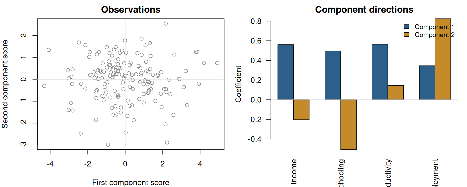
The first component assigns similar signs to income, schooling, productivity, and employment, reflecting their common latent factor in the simulated data. The second component distinguishes labour-market variation from the broader development direction. These interpretations are properties of this particular data-generating process, not general definitions of the first and second components.
Low-rank approximation
Ordering the singular values makes it possible to retain the strongest layers and discard the rest. The rank-\(q\) approximation is
\[ X_q=\sum_{j=1}^q d_ju_jv_j^\top. \]
The Eckart-Young theorem states that \(X_q\) minimizes the reconstruction error among all matrices of rank at most \(q\). Under the Frobenius norm,
\[ \min_{\operatorname{rank}(B)\leq q}\lVert X-B\rVert_F^2 =\lVert X-X_q\rVert_F^2 =\sum_{j=q+1}^r d_j^2. \]
Under the operator norm, the minimum error is \(d_{q+1}\). The result gives a precise meaning to the claim that small singular directions contain less of the matrix. Removing them loses less squared variation than removing any other collection of directions of the same dimension.
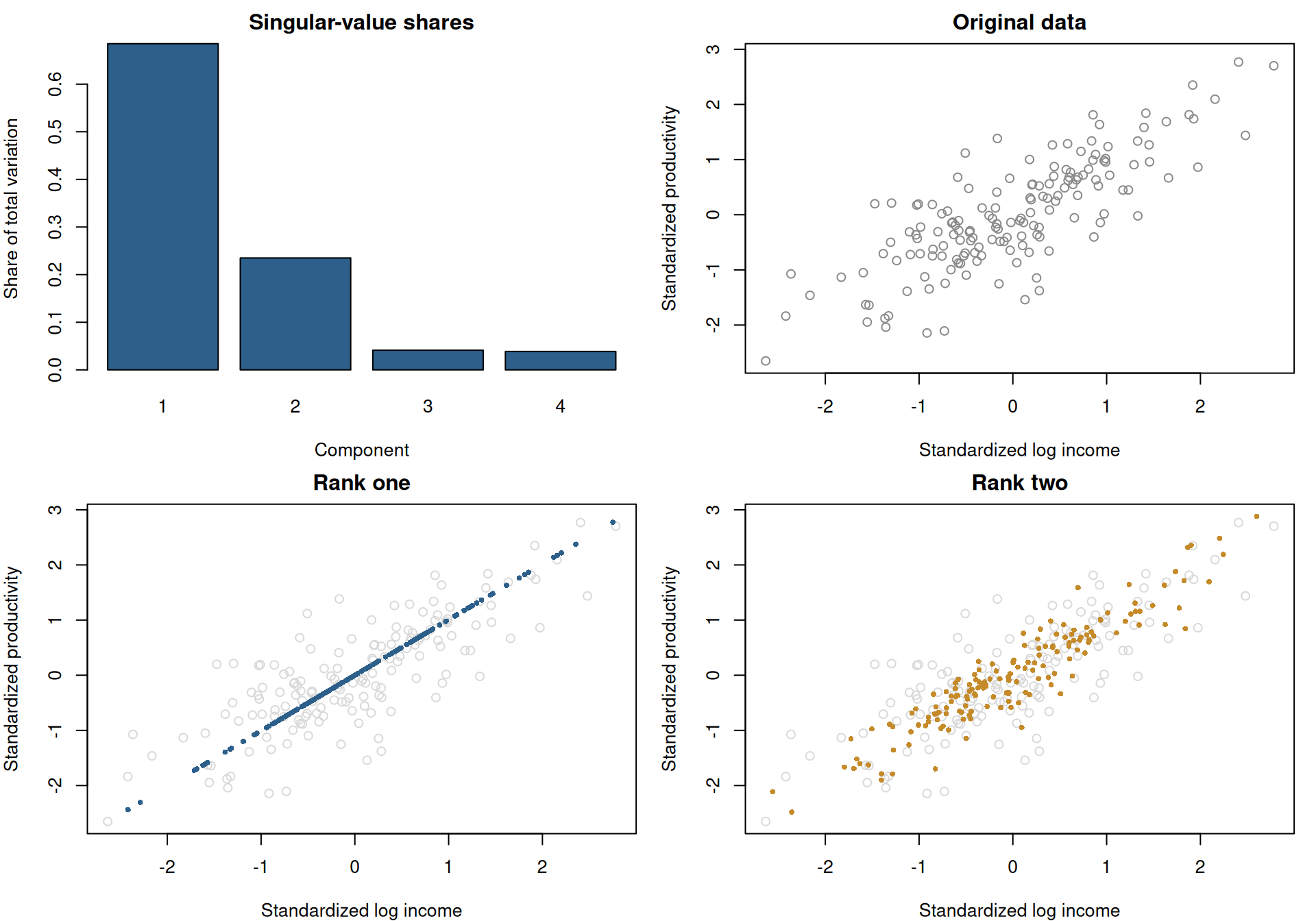
For this dataset, the first approximation places every observation on one line. The second allows a second independent direction and recovers most of the visible cloud. In empirical work, the appropriate rank cannot be selected from a picture alone. It depends on the purpose of the approximation, the amount of sampling noise, and the consequences of discarding variation.
Least squares and multicollinearity
The same decomposition clarifies linear regression. Here \(X\in\mathbb R^{N\times k}\) is the design matrix and \(y\in\mathbb R^N\) is the outcome vector; any intercept can be included as a column of ones, or handled separately when both \(X\) and \(y\) are centered. Ordinary least squares minimizes \(\lVert y-X\beta\rVert^2\). Setting the derivative with respect to \(\beta\) to zero gives the normal equations \(X^\top X\widehat\beta=X^\top y\). When \(X\) has full column rank, \(X^\top X\) is invertible, giving the familiar formula
\[ \widehat\beta=(X^\top X)^{-1}X^\top y. \]
The SVD expression is this same estimator written in different coordinates. Substitute the thin SVD \(X=UDV^\top\), where \(U^\top U=I_k\), \(V^\top V=VV^\top=I_k\), and all \(d_j>0\). Then
\[ X^\top X=VD^2V^\top, \qquad (X^\top X)^{-1}=VD^{-2}V^\top, \]
and therefore
\[ \begin{aligned} \widehat\beta &=(VD^{-2}V^\top)(VDU^\top)y\\ &=VD^{-1}U^\top y =\sum_{j=1}^k\frac{u_j^\top y}{d_j}v_j. \end{aligned} \]
The sequence reverses the fitted-value mapping \(\beta\mapsto X\beta=UDV^\top\beta\). First, \(U^\top y\) measures the outcome’s coordinates along the orthonormal directions spanning the column space of \(X\). Next, \(D^{-1}\) divides each coordinate by the amount that \(X\) stretches that direction. Finally, \(V\) combines those recovered coordinates into coefficients in the original variable basis. Because \(U\) is rectangular, \(U^\top y\) describes only the component of \(y\) in the column space: the fitted values are \(X\widehat\beta=UU^\top y\), and the residual \((I_N-UU^\top)y\) is perpendicular to every column of \(X\).
A small \(d_j\) consequently magnifies small changes in \(u_j^\top y\). Under homoskedastic errors with variance \(\sigma_\varepsilon^2\),
\[ \operatorname{Var}(\widehat\beta\mid X) =\sigma_\varepsilon^2VD^{-2}V^\top. \]
After the columns have been placed on comparable scales, near multicollinearity appears as a small singular value relative to the largest one. It means that some linear combination of columns is close to zero, so the data contain little information about the corresponding coefficient direction. The condition number \(d_1/d_r\) summarizes the disparity between the strongest and weakest identified directions.
Figure 10 uses two almost identical standardized regressors. Their condition number is approximately 56. Repeated small perturbations of the outcome generate large movements in the individual coefficients. The estimates move in opposite directions, leaving their sum and the fitted values much more stable.
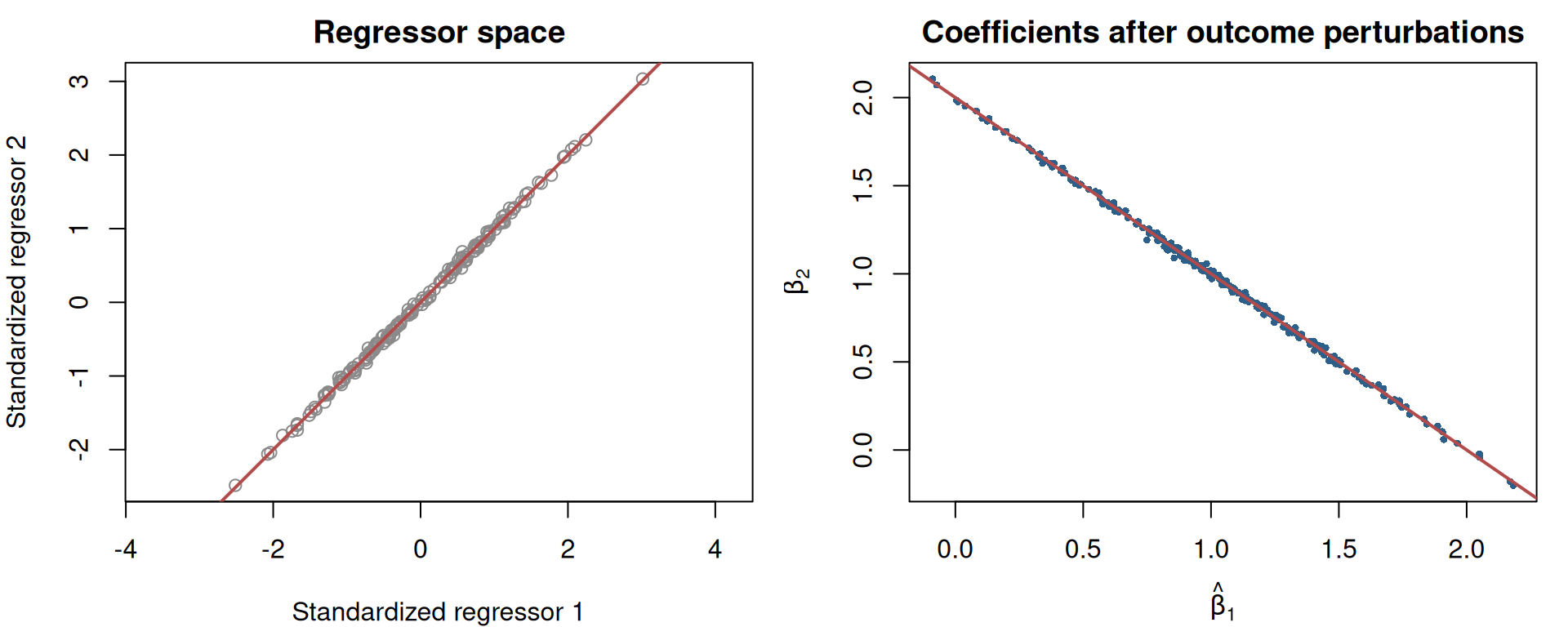
When \(X\) is rank deficient, the traditional inverse \((X^\top X)^{-1}\) does not exist. Retain only the \(r\) positive singular values and their vectors, writing \(X=U_rD_rV_r^\top\). The Moore-Penrose pseudoinverse and its coefficient estimate are
\[ X^+=V_rD_r^{-1}U_r^\top, \qquad \widehat\beta^+=X^+y =\sum_{j=1}^r\frac{u_j^\top y}{d_j}v_j. \]
This still minimizes the residual sum of squares, since \(X\widehat\beta^+=U_rU_r^\top y\) is the orthogonal projection onto the column space of \(X\). Every other least-squares solution is \(\widehat\beta^++z\) for some \(z\) in the null space of \(X\). The vector \(\widehat\beta^+\) lies in the span of \(v_1,\ldots,v_r\), which is perpendicular to that null space, so
\[ \lVert\widehat\beta^++z\rVert^2 =\lVert\widehat\beta^+\rVert^2+\lVert z\rVert^2. \]
The pseudoinverse therefore selects the least-squares solution with minimum Euclidean norm. This does not create information in a missing direction; it supplies a well-defined representative among observationally equivalent coefficient vectors. The SVD separates that identification issue from the directions that the data estimate precisely.
Conclusion
The singular value decomposition describes a matrix through matched orthogonal directions. The columns of \(V\) identify input directions, the singular values state how strongly the matrix acts along them, and the columns of \(U\) identify the resulting output directions. The decomposition exists because \(A^\top A\) is a real symmetric positive-semidefinite matrix whose orthonormal eigenvectors provide the required input basis.
For a centered data matrix, the same objects have statistical interpretations. The right singular vectors are principal-component directions, \(UD\) contains observation scores, and squared singular values determine the variance along each component. Retaining the largest singular layers gives the best low-rank approximation. In regression, inverting those layers reveals why weak singular directions produce unstable coefficients. These are different uses of one construction: a matrix becomes transparent once its action is expressed in the directions it treats independently.
Footnotes
Perpendicularity of the \(v_j\) follows from the eigenvectors used to construct them. The existence proof below takes the \(v_j\) to be eigenvectors of \(B=A^\top A\), which is symmetric. For a real symmetric \(B\) with \(Bv_i=\lambda_iv_i\) and \(Bv_j=\lambda_jv_j\), moving \(B\) across the inner product gives \(\lambda_iv_i^\top v_j=(Bv_i)^\top v_j=v_i^\top Bv_j=\lambda_jv_i^\top v_j\), so \((\lambda_i-\lambda_j)v_i^\top v_j=0\). Whenever the two eigenvalues differ, the second factor must vanish and the eigenvectors are perpendicular. If an eigenvalue is repeated, its eigenspace has dimension larger than one and perpendicularity is no longer automatic, but any basis of that eigenspace can be replaced by an orthonormal one, and the replacement remains in the eigenspace because a subspace is closed under linear combinations. Unit length is a normalization: an eigenvector is determined only up to scale, so each is divided by its own length.↩︎
The \(u_j\) inherit their perpendicularity from the \(v_j\) through the definition \(u_j=Av_j/\sigma_j\), which the existence proof below uses for every direction with \(\sigma_j>0\). Substituting that definition and using \(A^\top Av_j=\lambda_jv_j\) with \(\lambda_j=\sigma_j^2\) gives \(u_i^\top u_j=v_i^\top A^\top Av_j/(\sigma_i\sigma_j)=\lambda_jv_i^\top v_j/(\sigma_i\sigma_j)\). For \(i\neq j\) this is zero because \(v_i^\top v_j=0\), and for \(i=j\) it is \(\lambda_j/\sigma_j^2=1\). The images of perpendicular input directions are therefore perpendicular themselves, although \(A\) does not preserve angles between arbitrary directions. Columns of \(U\) associated with a zero singular value are not obtained this way; they are chosen directly as an orthonormal basis of the orthogonal complement of the column space of \(A\).↩︎
A real square matrix \(Q\) is orthogonal when \(Q^\top Q=I\). For any vectors \(a,b\), \((Qa)^\top(Qb)=a^\top Q^\top Qb=a^\top b\), so dot products are preserved. Setting \(a=b\) gives \(\|Qa\|^2=\|a\|^2\). For nonzero vectors the angle is determined by \(\cos\theta=(a^\top b)/(\|a\|\|b\|)\), whose numerator and denominator are both preserved. This applies to \(Q=U\) and \(Q=V^\top\) in the full SVD, since \(U^\top U=I\) and \(VV^\top=I\).↩︎