Constrained optimization, duality, and support vector machines

Introduction

A support vector machine (SVM) chooses a separating hyperplane by solving a constrained optimization problem. The geometry is simple: among all hyperplanes that classify a linearly separable training sample correctly, it selects the one with the largest distance to the closest observations. The optimization is also useful beyond this particular classifier. It illustrates why Lagrange multipliers are introduced, how constraints become a dual problem, and why a method that starts with linear boundaries can use nonlinear features through a kernel.

Let the training sample contain \(n\) observations. Observation \(i\) has a feature vector \(x_i\in\mathbb{R}^{p}\) and a binary label \(y_i\in\{-1,+1\}\). The vectors are columns, so \(w\in\mathbb{R}^{p}\) is also a column vector and \(w^\top x_i\) is a scalar. The classifier is based on the affine score

\[ f(x)=w^\top x+b, \]

where \(b\in\mathbb{R}\) is an intercept. It predicts \(+1\) when \(f(x)>0\) and \(-1\) when \(f(x)<0\). Its decision boundary is the hyperplane \(\{x:w^\top x+b=0\}\). The companion note on affine hyperplanes derives that the distance from a point \(x\) to this hyperplane is \(|w^\top x+b|/\lVert w\rVert_2\) when \(w\ne0\).

This note first formulates the hard-margin SVM, then derives its dual and states the conditions under which the two problems have the same solution value. It subsequently allows classification errors through slack variables and shows the equivalent hinge-loss problem. The final section replaces ordinary inner products by a positive-semidefinite kernel.

The hard-margin problem

Correct classification of training observation \(i\) means that \(f(x_i)\) has the same sign as \(y_i\). Multiplying the score by its label expresses both classes with one inequality:

\[ y_i(w^\top x_i+b)>0. \]

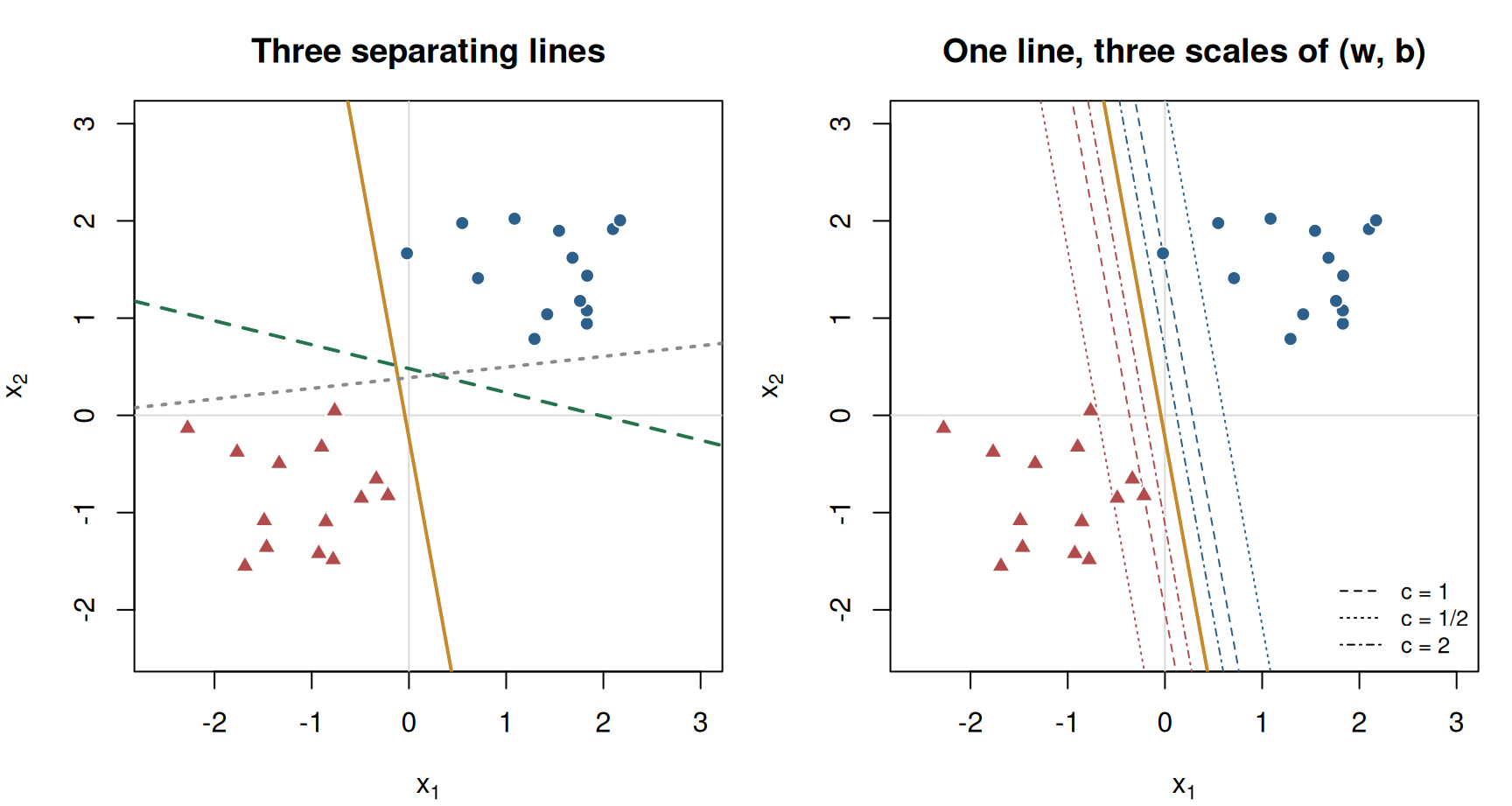
If \(y_i=+1\), this requires \(w^\top x_i+b>0\). If \(y_i=-1\), it requires \(w^\top x_i+b<0\). The condition alone does not select one separating hyperplane. In particular, multiplying both \(w\) and \(b\) by any positive number changes the numerical score but leaves the boundary, and all predicted signs, unchanged. Figure 1 illustrates both points for a synthetic sample of 28 observations in two dimensions.

Figure 1: Separation does not determine a unique hyperplane, and a hyperplane does not determine a unique scale. Blue circles have \(y_i=+1\) and red triangles have \(y_i=-1\). Left: three lines, each of which satisfies \(y_i(w^\top x_i+b)>0\) for all 28 observations. Each line is drawn halfway across the gap between the two classes in its own normal direction, so none of them is arbitrary, yet they differ substantially in orientation. Right: the solid gold line is the first of the three boundaries, \(w^\top x+b=0\). The dashed, dotted, and dash-dotted pairs are the level sets \(c(w^\top x+b)=\pm1\) for \(c=1\), \(c=1/2\), and \(c=2\); blue lines have value \(+1\) and red lines \(-1\). Multiplying \((w,b)\) by \(c\) leaves the boundary unchanged but moves the lines \(\pm1\) to distance \(1/(c\lVert w\rVert_2)\) from it. At \(c=1\) the scale is chosen so that the closest observation has \(y_i(w^\top x_i+b)=1\) exactly and lies on a dashed line. At \(c=1/2\) that observation has value \(1/2\) and violates the normalized constraint; at \(c=2\) no observation touches the dash-dotted lines.

The SVM uses this freedom of scale to set the score of the closest correctly classified observations equal to one:

\[ y_i(w^\top x_i+b)\geq1, \qquad i=1,\ldots,n. \]

The two parallel supporting hyperplanes are consequently \(w^\top x+b=1\) and \(w^\top x+b=-1\). Each is \(1/\lVert w\rVert_2\) away from the decision boundary, so their distance is \(2/\lVert w\rVert_2\). Maximising the distance to the closest training observation is therefore equivalent to minimising \(\lVert w\rVert_2\). Squaring the norm and multiplying by one half do not change the minimiser, and give a convenient derivative. The hard-margin primal problem is

\[ \begin{aligned} \min_{w\in\mathbb{R}^{p},\,b\in\mathbb{R}} \quad & \frac{1}{2}\lVert w\rVert_2^2\\ \text{subject to}\quad &y_i(w^\top x_i+b)\geq1, \qquad i=1,\ldots,n. \end{aligned} \tag{P} \]

This problem is feasible only when the two classes can be separated by a hyperplane. It is a convex optimization problem: its objective is a convex quadratic function of \(w\), and each constraint describes a half-space in the joint parameter \((w,b)\). Convexity matters because a feasible local minimum is then a global minimum. It does not yet by itself establish the dual representation derived below; that conclusion also uses strong duality.

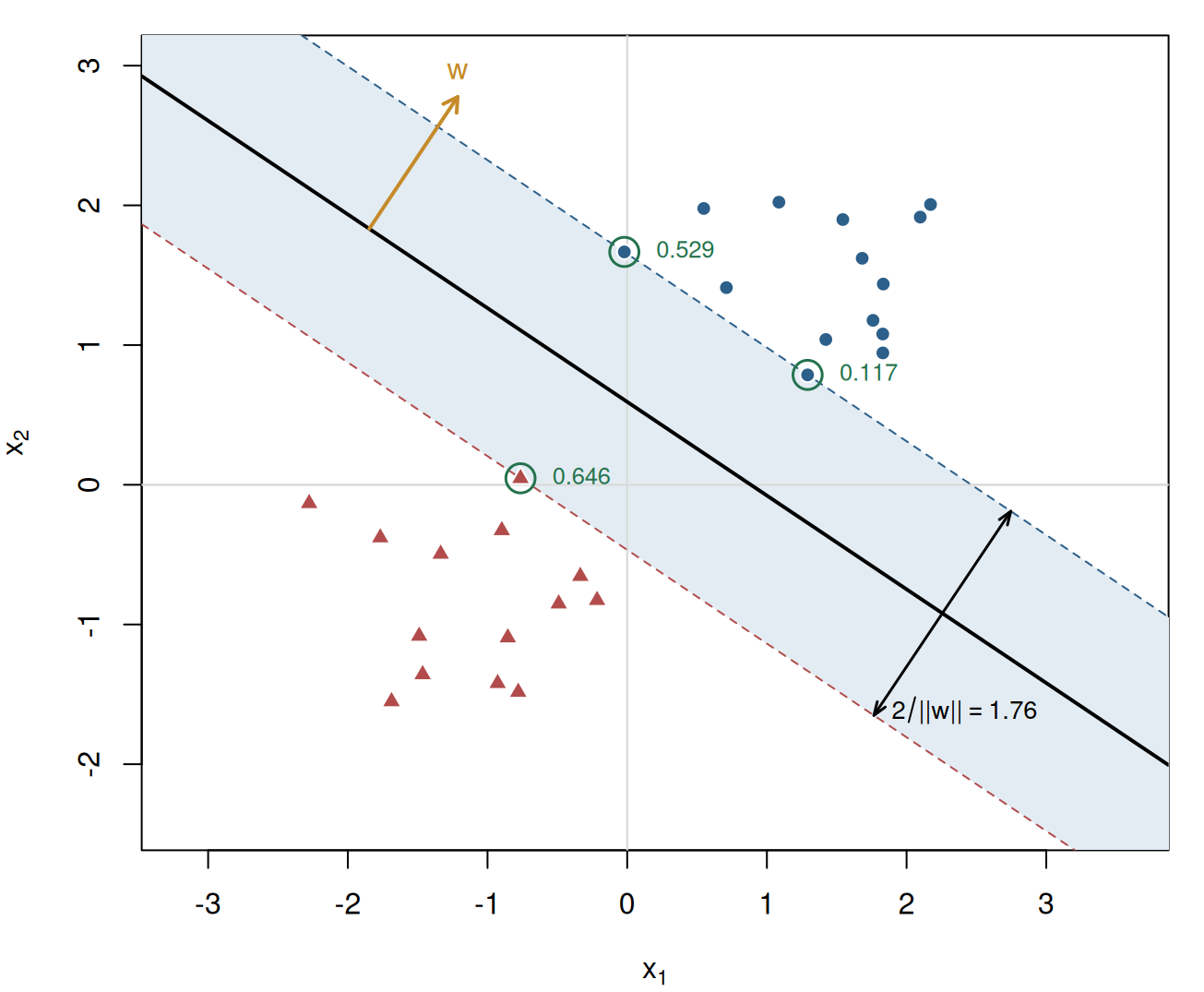
Figure 2 shows the solution of (P) for the sample in Figure 1. The fitted normal vector is \(w\approx(0.633,0.944)^\top\), so the distance between the two supporting hyperplanes is \(2/\lVert w\rVert_2\approx1.76\). Three observations lie on those hyperplanes. No other separating line in the plane leaves a wider gap between the classes.

Figure 2: The hard-margin solution for the 28 observations in the preceding figure. The solid black line is the decision boundary \(w^\top x+b=0\). The dashed blue and red lines are the supporting hyperplanes \(w^\top x+b=+1\) and \(w^\top x+b=-1\), and the shaded band between them contains no observations. The gold arrow is \(w\approx(0.633,0.944)^\top\), drawn from a point on the boundary; it is perpendicular to all three lines and points towards the class \(y=+1\). The double-headed black arrow measures the margin width \(2/\lVert w\rVert_2\approx1.76\) along \(w\). The three circled observations are the only ones with positive dual coefficients, and the printed numbers are their values of \(\alpha_i\). The two blue coefficients sum to \(0.117+0.529=0.646\), which equals the red coefficient, as the constraint \(\sum_i\alpha_i y_i=0\) in (1) requires.

Lagrange multipliers and the dual problem

Each inequality in (P) restricts the allowed \((w,b)\). A non-negative Lagrange multiplier \(\alpha_i\geq0\) records the role of constraint \(i\). To use the conventional less-than-or-equal-to-zero form, write the constraint as

\[ g_i(w,b)=1-y_i(w^\top x_i+b)\leq0. \]

The Lagrangian is the objective plus a weighted sum of these constraint functions:

\[ \begin{aligned} \mathcal{L}(w,b,\alpha) &=\frac{1}{2}w^\top w +\sum_{i=1}^{n}\alpha_i\left[1-y_i(w^\top x_i+b)\right]\\ &=\frac{1}{2}w^\top w -w^\top\sum_{i=1}^{n}\alpha_i y_i x_i -b\sum_{i=1}^{n}\alpha_i y_i +\sum_{i=1}^{n}\alpha_i. \end{aligned} \]

The second line only collects the terms containing \(w\), \(b\), and neither parameter. It also makes clear why the multipliers must be non-negative. At a feasible \((w,b)\), every \(g_i(w,b)\) is non-positive. Thus adding \(\alpha_i g_i(w,b)\) cannot increase the objective when \(\alpha_i\geq0\).

For fixed multipliers, the dual function is the smallest value of the Lagrangian over the unconstrained primal parameters,

\[ q(\alpha)=\inf_{w,b}\mathcal{L}(w,b,\alpha). \]

To obtain a finite infimum, first differentiate with respect to \(b\). Since \(b\) occurs only in \(-b\sum_i\alpha_i y_i\),

\[ \frac{\partial\mathcal{L}}{\partial b} =-\sum_{i=1}^{n}\alpha_i y_i=0. \]

If this equality did not hold, the Lagrangian would be a nonconstant linear function of \(b\) and could be made arbitrarily negative by sending \(b\) in one direction or the other. Hence a finite dual value requires

\[ \sum_{i=1}^{n}\alpha_i y_i=0. \tag{1} \]

The derivative with respect to \(w\) is

\[ \frac{\partial\mathcal{L}}{\partial w} =w-\sum_{i=1}^{n}\alpha_i y_i x_i. \]

Setting it to zero gives the minimizing weight vector for the specified multipliers,

\[ w=\sum_{i=1}^{n}\alpha_i y_i x_i. \tag{2} \]

Let \(s=\sum_i\alpha_i y_i x_i\). Under (1), the term involving \(b\) vanishes, and substituting \(w=s\) into the Lagrangian gives

\[ \begin{aligned} q(\alpha) &=\frac{1}{2}s^\top s-s^\top s+\sum_{i=1}^{n}\alpha_i\\ &=\sum_{i=1}^{n}\alpha_i -\frac{1}{2}\left\lVert\sum_{i=1}^{n}\alpha_i y_i x_i\right\rVert_2^2\\ &=\sum_{i=1}^{n}\alpha_i -\frac{1}{2}\sum_{i=1}^{n}\sum_{j=1}^{n} \alpha_i\alpha_jy_i y_jx_i^\top x_j. \end{aligned} \]

The final line expands the squared norm. It exposes a central fact: the observations enter the dual only through pairwise inner products. The hard-margin dual problem is therefore

\[ \begin{aligned} \max_{\alpha\in\mathbb{R}^{n}} \quad & \sum_{i=1}^{n}\alpha_i -\frac{1}{2}\sum_{i=1}^{n}\sum_{j=1}^{n} \alpha_i\alpha_jy_i y_jx_i^\top x_j\\ \text{subject to}\quad &\alpha_i\geq0,\qquad i=1,\ldots,n,\\ &\sum_{i=1}^{n}\alpha_i y_i=0. \end{aligned} \tag{D} \]

For arbitrary feasible multipliers, \(q(\alpha)\) is a lower bound on the primal optimum. This is weak duality. For a linearly separable finite sample, a strictly feasible version of (P) exists after rescaling a separating \((w,b)\) so that every left-hand side exceeds one. The objective and constraints are convex, so this strict feasibility condition, called Slater’s condition, implies strong duality. The optimum values of (P) and (D) are then equal, and their optimizers satisfy the conditions in the next section. This use of strong duality is an additional convex-optimization result; it does not follow merely from differentiating the Lagrangian.

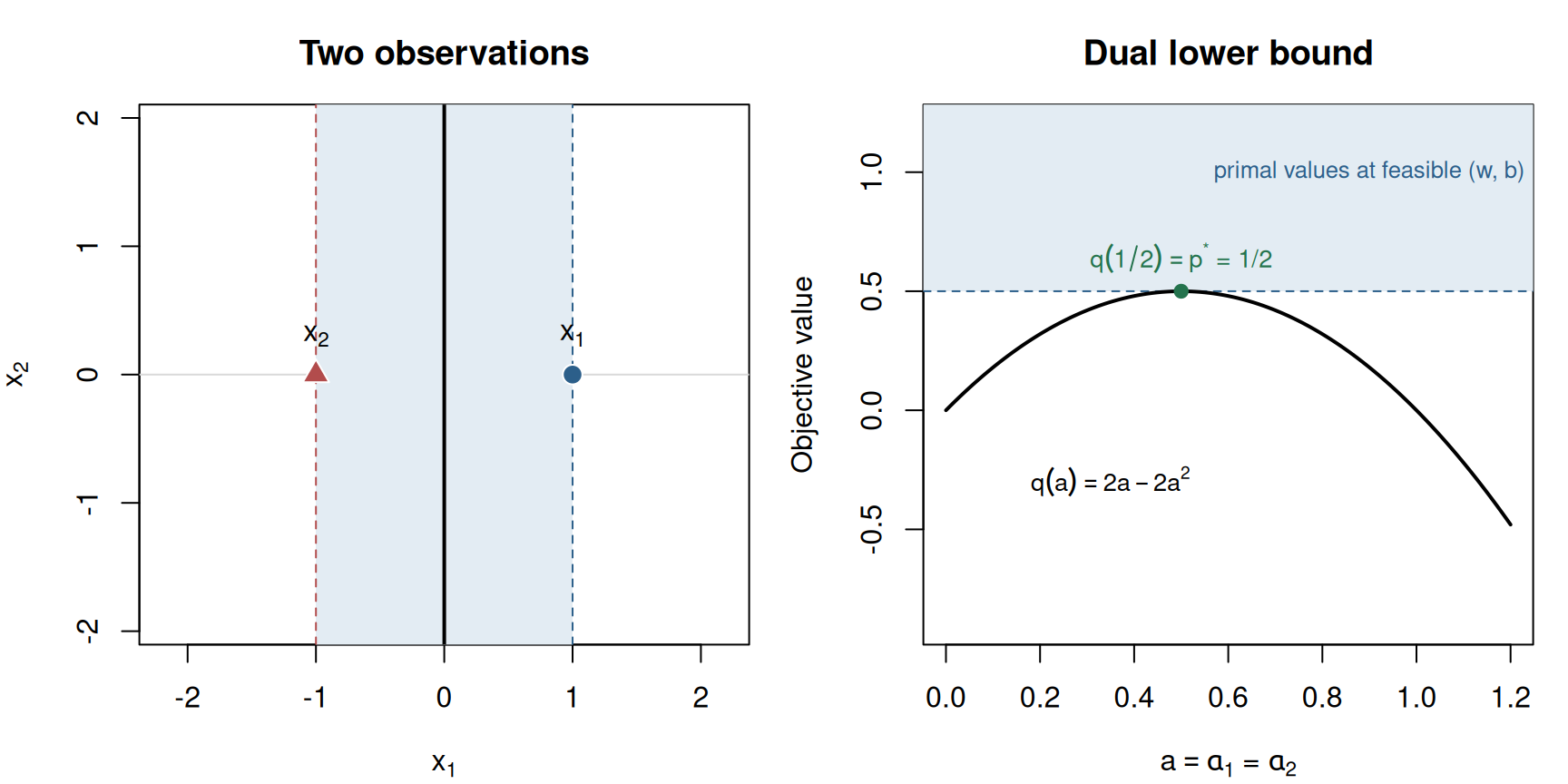
A sample of two observations makes both statements visible. Let \(x_1=(1,0)^\top\) with \(y_1=+1\) and \(x_2=(-1,0)^\top\) with \(y_2=-1\). The primal constraints are \(w_1+b\geq1\) and \(w_1-b\geq1\). Adding them gives \(w_1\geq1\), so every feasible \((w,b)\) has \(\frac{1}{2}\lVert w\rVert_2^2\geq\frac{1}{2}\), and \(w=(1,0)^\top\), \(b=0\) attains this bound. On the dual side, (1) requires \(\alpha_1=\alpha_2=a\), and (2) gives \(w=a x_1-a x_2=(2a,0)^\top\). The dual objective is then \(q(a)=2a-\frac{1}{2}(2a)^2=2a-2a^2\). Figure 3 plots both sides of the comparison.

Figure 3: Weak and strong duality for two observations. Left: the observations \(x_1=(1,0)^\top\) with \(y_1=+1\) and \(x_2=(-1,0)^\top\) with \(y_2=-1\), the optimal boundary, which is the vertical axis, and the supporting hyperplanes through the two observations. Right: the black curve is the dual objective \(q(a)=2a-2a^2\) along the feasible dual set \(\alpha_1=\alpha_2=a\geq0\). The shaded region above the dashed line contains every value \(\frac{1}{2}\lVert w\rVert_2^2\) attained by a feasible \((w,b)\); its lower edge is the primal optimum \(p^\ast=\frac{1}{2}\). The curve never enters the shaded region, which is weak duality: every dual value is a lower bound on every primal value. The curve touches the region at \(a=\frac{1}{2}\), where \(q=p^\ast\); this is strong duality. Substituting \(a=\frac{1}{2}\) in (2) gives \(w=(1,0)^\top\), the primal solution.

KKT conditions and support vectors

Under strong duality, a primal-dual optimum \((w,b,\alpha)\) satisfies the Karush–Kuhn–Tucker (KKT) conditions:

\[ \begin{array}{rll} \text{primal feasibility:}&y_i(w^\top x_i+b)&\geq1,\\ \text{dual feasibility:}&\alpha_i&\geq0,\\ \text{stationarity:}&w&=\sum_{i=1}^{n}\alpha_i y_i x_i,\\ &&\sum_{i=1}^{n}\alpha_i y_i=0,\\ \text{complementary slackness:}&\alpha_i\,[y_i(w^\top x_i+b)-1]&=0, \end{array} \qquad i=1,\ldots,n. \]

The first two lines repeat the constraints of the primal and dual. Stationarity repeats the two derivatives set to zero above. Complementary slackness links a multiplier to the associated training observation. If observation \(i\) lies strictly beyond its supporting hyperplane, so that \(y_i(w^\top x_i+b)>1\), the bracket is positive and complementary slackness forces \(\alpha_i=0\). Such an observation does not appear in (2). If \(\alpha_i>0\), it must instead lie exactly on its class’s supporting hyperplane. These observations are the support vectors in the dual representation, because they alone determine \(w\). Figure 4 verifies both statements for the sample in Figure 2.

Figure 4: Complementary slackness and the representation (2) for the hard-margin solution in the earlier figure. Left: each of the 28 observations plotted by its functional margin \(y_i f(x_i)\) and its dual coefficient \(\alpha_i\). No point lies to the left of the dashed line at \(1\), which is primal feasibility. Every point with \(y_i f(x_i)>1\) has \(\alpha_i=0\), and the three circled points with \(\alpha_i>0\) all have \(y_i f(x_i)=1\), so the product \(\alpha_i[y_i f(x_i)-1]\) is zero for every observation. Right: the three nonzero terms \(\alpha_i y_i x_i\) of (2), placed head to tail in the order of their coefficients \(0.117\), \(0.529\), and \(0.646\). Blue arrows come from observations with \(y_i=+1\) and point in the direction of \(x_i\); the red arrow comes from an observation with \(y_i=-1\) and therefore points in the direction of \(-x_i\). The dashed gold arrow from the origin is \(w\approx(0.633,0.944)^\top\) computed by the solver, and it ends where the three terms end. The remaining 25 observations contribute nothing to the sum.

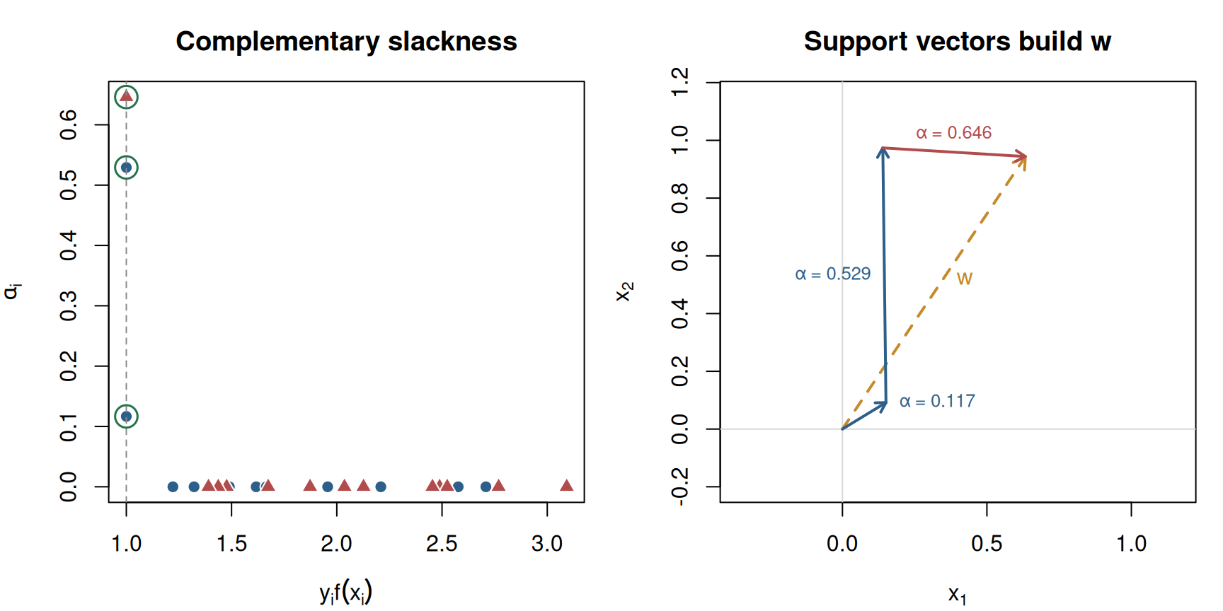
There can be a training observation on a supporting hyperplane with coefficient zero, for example when the solution is not unique in its coefficients. Geometric usage sometimes calls it a support vector as well. The more precise statement for the calculation is that positive coefficients identify the observations that enter (2).

Once \(w\) is known, any training observation with \(\alpha_i>0\) yields an intercept in the hard-margin case:

\[ b=y_i-w^\top x_i. \]

This follows from its equality \(y_i(w^\top x_i+b)=1\) and \(y_i^2=1\). Numerical implementations commonly average this expression over suitable support vectors, because finite-precision optimization can make the individual values differ slightly.

Soft margins and hinge loss

Real data are often not linearly separable. A soft-margin SVM introduces a non-negative slack variable \(\xi_i\) for every observation:

\[ \begin{aligned} \min_{w,b,\xi}\quad &\frac{1}{2}\lVert w\rVert_2^2+C\sum_{i=1}^{n}\xi_i\\ \text{subject to}\quad &y_i(w^\top x_i+b)\geq1-\xi_i, \qquad i=1,\ldots,n,\\ &\xi_i\geq0, \qquad i=1,\ldots,n, \end{aligned} \tag{$\mathrm{P}_{\mathrm{soft}}$} \]

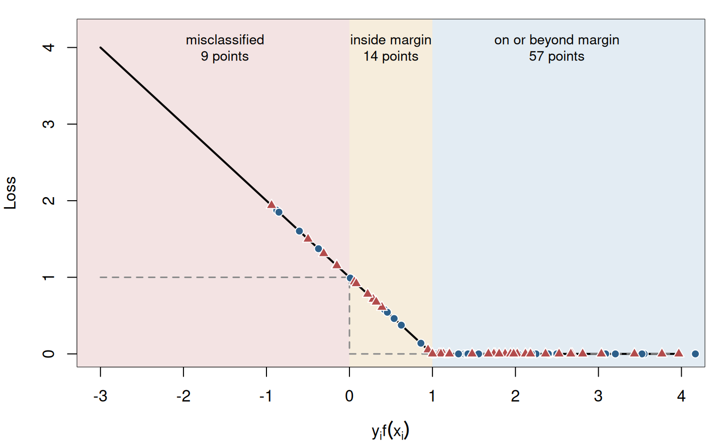
where \(C>0\) determines the relative penalty for margin violations. A point with \(\xi_i=0\) is correctly classified and on or beyond the margin. A point with \(0<\xi_i\leq1\) is correctly classified but lies inside the margin. A point with \(\xi_i>1\) has \(y_i f(x_i)<0\) and is misclassified. The problem remains convex: the objective is convex and all constraints are affine. It also has a strictly feasible point for any sample, for example \(w=0\), \(b=0\), and every \(\xi_i=2\). Thus Slater’s condition, and hence strong duality, apply without a separability assumption.

To derive the soft-margin dual, add a multiplier \(\alpha_i\geq0\) for \(1-\xi_i-y_i(w^\top x_i+b)\leq0\) and a multiplier \(\mu_i\geq0\) for \(-\xi_i\leq0\). The new terms in the Lagrangian are

\[ \sum_{i=1}^{n}\alpha_i[1-\xi_i-y_i(w^\top x_i+b)] -\sum_{i=1}^{n}\mu_i\xi_i. \]

Differentiation with respect to \(w\) and \(b\) gives the same two stationarity equations (1) and (2). Differentiation with respect to \(\xi_i\) gives

\[ C-\alpha_i-\mu_i=0. \]

Since both multipliers are non-negative, this equality is equivalent to \(0\leq\alpha_i\leq C\). Substituting the stationarity equations gives the same quadratic dual objective as before, now with box constraints:

\[ \begin{aligned} \max_{\alpha\in\mathbb{R}^{n}} \quad & \sum_{i=1}^{n}\alpha_i -\frac{1}{2}\sum_{i=1}^{n}\sum_{j=1}^{n} \alpha_i\alpha_jy_i y_jx_i^\top x_j\\ \text{subject to}\quad &0\leq\alpha_i\leq C,\qquad i=1,\ldots,n,\\ &\sum_{i=1}^{n}\alpha_i y_i=0. \end{aligned} \tag{$\mathrm{D}_{\mathrm{soft}}$} \]

The soft-margin KKT conditions add \(\mu_i\xi_i=0\) and replace the hard-margin constraint by \(y_i f(x_i)\geq1-\xi_i\). In a non-degenerate solution, coefficients strictly between zero and \(C\) identify points on the margin with zero slack. A coefficient at \(C\) can identify a point inside the margin or misclassified. The qualification is useful because boundary cases can also occur when a point is exactly on the margin.

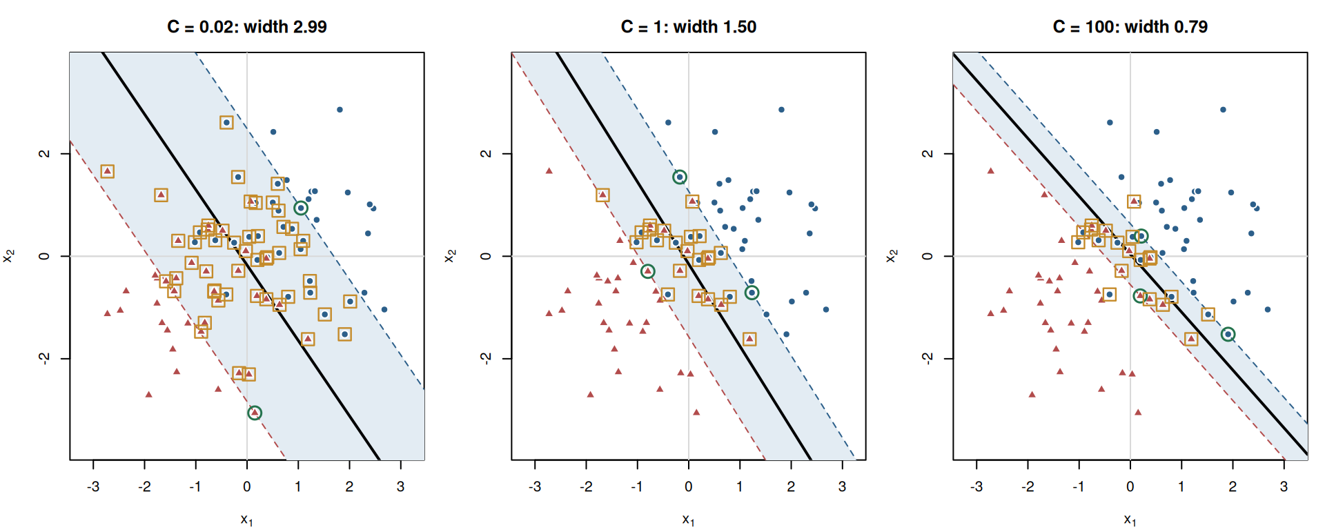
Figure 5 applies the soft-margin problem to 80 observations from two overlapping classes, which no line can separate. The three panels differ only in \(C\). A small penalty tolerates many margin violations and chooses a wide band: at \(C=0.02\), 54 of the 80 observations have positive coefficients. As \(C\) grows, violations become more expensive, the band narrows, and fewer observations enter (2). The training error changes much less than the margin width, from 11.2 to 10.0 percent.

Figure 5: Soft-margin solutions for the same 80 observations at three values of the penalty \(C\). Blue circles have \(y_i=+1\) and red triangles \(y_i=-1\). In each panel the solid line is \(f(x)=0\), the dashed lines are \(f(x)=\pm1\), and the shaded band between them has width \(2/\lVert w\rVert_2\), printed above the panel. Green circles mark observations with \(0<\alpha_i<C\); complementary slackness places them exactly on a dashed line with \(\xi_i=0\). Gold squares mark observations with \(\alpha_i=C\); these lie on the wrong side of their own dashed line, inside the band or beyond the boundary, with \(\xi_i>0\). Unmarked observations have \(\alpha_i=0\) and lie on or beyond their dashed line. The number of observations with \(\alpha_i>0\) falls from 54 at \(C=0.02\) to 26 at \(C=1\) and 23 at \(C=100\), while the width falls from 2.99 to 1.50 and 0.79.

The slack variables can be removed from the primal. For fixed \((w,b)\), the two constraints require

\[ \xi_i\geq 0 \qquad\text{and}\qquad \xi_i\geq1-y_i f(x_i). \]

The objective increases with \(\xi_i\), so its smallest allowed value is

\[ \xi_i=\max\{0,1-y_i f(x_i)\}. \]

This maximum is the hinge loss, written \(\ell_{\mathrm{hinge}}(y_i,f(x_i))\). Substitution gives the unconstrained formulation

\[ \min_{w,b}\quad \frac{1}{2}\lVert w\rVert_2^2 +C\sum_{i=1}^{n}\max\{0,1-y_i(w^\top x_i+b)\}. \]

The loss is zero when an observation is correctly classified with a margin of at least one. It grows linearly when the observation enters the margin and continues to grow after misclassification. The norm penalty still favours a wide boundary, whereas \(C\) determines how much violation of the training margins can be traded for that width. Figure 6 plots the loss together with the fitted slack values from the middle panel of Figure 5.

Figure 6: Hinge loss as a function of the functional margin \(y_i f(x_i)\). The solid black line is \(\max\{0,1-y_i f(x_i)\}\); the dashed grey step is the misclassification indicator, equal to one when \(y_i f(x_i)<0\). The hinge loss lies on or above this indicator everywhere, so the sum of slacks bounds the number of training errors. The points are the 80 observations from the soft-margin fit with \(C=1\), each placed at its fitted margin and its optimal slack \(\xi_i\). All of them lie on the hinge, which is the elimination argument of the text: at the optimum each slack equals its hinge loss. The shaded regions follow the three cases for \(\xi_i\). In the blue region \(\xi_i=0\) (57 observations), in the pale gold region \(0<\xi_i\leq1\) and the observation is correctly classified inside the margin (14 observations), and in the red region \(\xi_i>1\) and the observation is misclassified (9 observations).

Kernel SVMs

The dual objective and prediction rule require inner products, not the individual coordinates of \(x_i\). Suppose that each observation is mapped to a feature vector \(\phi(x)\) in some inner-product space. Applying the preceding soft-margin SVM to \(\phi(x_i)\) replaces every occurrence of \(x_i^\top x_j\) with

\[ k(x_i,x_j)=\phi(x_i)^\top\phi(x_j). \]

The function \(k\) is called a kernel. For the training sample, collect these pairwise values in the \(n\times n\) kernel Gram matrix \(K\), where \(K_{ij}=k(x_i,x_j)\). It must be symmetric and positive semidefinite:

\[ a^\top K a\geq0 \qquad\text{for every }a\in\mathbb{R}^{n}. \]

The condition is necessary when \(K\) is formed from feature inner products, because \(a^\top K a=\lVert\sum_i a_i\phi(x_i)\rVert_2^2\). It is also sufficient for a finite training matrix: an eigendecomposition of a PSD \(K\) constructs vectors with that Gram matrix. A kernel function is ordinarily required to produce such a matrix for every finite set of possible inputs, so that it consistently represents an inner product in some feature space.

With a valid kernel, the soft-margin dual becomes

\[ \begin{aligned} \max_{\alpha\in\mathbb{R}^{n}} \quad & \sum_{i=1}^{n}\alpha_i -\frac{1}{2}\sum_{i=1}^{n}\sum_{j=1}^{n} \alpha_i\alpha_jy_i y_jK_{ij}\\ \text{subject to}\quad &0\leq\alpha_i\leq C,\qquad i=1,\ldots,n,\\ &\sum_{i=1}^{n}\alpha_i y_i=0. \end{aligned} \]

For a new observation \(x\), the score is obtained without explicitly constructing \(\phi(x)\):

\[ f(x)=\sum_{i=1}^{n}\alpha_i y_i k(x_i,x)+b. \]

This equality follows by substituting \(w=\sum_i\alpha_i y_i\phi(x_i)\) into \(w^\top\phi(x)+b\). Only support vectors with positive coefficients contribute to the sum. A polynomial kernel, \(k(x,z)=(x^\top z+c)^d\) for suitable \(c\) and integer \(d\), corresponds to interactions and powers of the original coordinates. The radial basis function kernel, \(k(x,z)=\exp(-\gamma\lVert x-z\rVert_2^2)\) with \(\gamma>0\), gives a similarity that falls as two observations move apart. Both can yield a decision boundary that is nonlinear in the original coordinates even though the separating rule is linear in feature space.

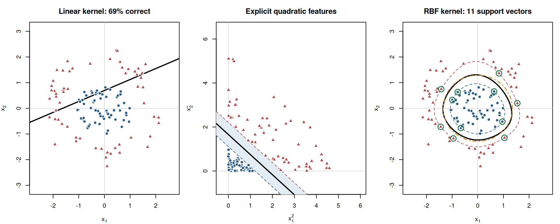
Figure 7 illustrates this with 120 observations, one class inside a disc and the other in a surrounding ring. A linear SVM in the original coordinates classifies only 69 percent of the training sample correctly, because no line separates a disc from a ring. The explicit map \(\phi(x)=(x_1^2,x_2^2)^\top\) uses two of the coordinates of the feature map of the quadratic kernel \((x^\top z)^2\). In these coordinates the classes are linearly separable, and the fitted line \(w^\top\phi(x)+b=0\) corresponds to the ellipse \(1.663x_1^2+1.823x_2^2=3.021\) in the original coordinates. The radial basis function kernel with \(\gamma=0.5\) and \(C=10\) never constructs a feature vector, yet its boundary is close to that ellipse and is determined by 11 support vectors.

Figure 7: A nonlinear boundary from a linear rule in feature space. The sample contains 60 observations with \(y_i=+1\) (blue circles) inside a disc of radius 1.1 and 60 with \(y_i=-1\) (red triangles) in a ring with radii between 1.5 and 2.4. Left: the linear SVM with \(C=1\) in the original coordinates; its boundary classifies 69 percent of the observations correctly. Middle: the same observations after the map \(\phi(x)=(x_1^2,x_2^2)^\top\), which sends the disc to a region near the origin and the ring to a band further out. The linear soft-margin SVM with \(C=10\) separates them, with the boundary as a solid line and the margins \(f=\pm1\) as dashed lines. Right: the RBF-kernel SVM with \(k(x,z)=\exp(-0.5\lVert x-z\rVert_2^2)\) and \(C=10\), fitted through the dual with the kernel matrix in place of \(x_i^\top x_j\). The solid black curve is \(f(x)=\sum_i\alpha_i y_i k(x_i,x)+b=0\), the dashed curves are \(f(x)=\pm1\), and the 11 circled observations have \(\alpha_i>0\); all other terms of the sum are zero. The dash-dotted gold curve is the boundary from the middle panel mapped back to the original coordinates, an ellipse with semiaxes of approximately 1.35 and 1.29. Both nonlinear boundaries classify every training observation correctly.

The kernel changes the representation of similarity, not the logic of the SVM. The margin is still determined by a norm in the feature space, the dual coefficients are still constrained by the labels and \(C\), and KKT conditions still identify which observations determine the fitted boundary. Kernel choice and feature scaling therefore remain substantive modelling decisions rather than automatic ways to improve classification.

Conclusion

The hard-margin SVM translates maximum-margin geometry into a convex quadratic program. Its Lagrangian and KKT conditions show that only observations on the supporting hyperplanes can enter the fitted normal vector, while the dual replaces the original coordinates with pairwise inner products. Slack variables extend the construction to nonseparable samples, and eliminating them produces hinge loss with a penalty controlled by \(C\). A positive-semidefinite kernel substitutes feature-space inner products for ordinary ones, preserving the same dual logic while allowing a nonlinear boundary in the original coordinates.