Democracy and peace
By Bas Machielsen
February 27, 2023
Introduction
I wanted to write a short post on democratic peace theory to simply explore the correlation between democracy and peace. It is sometimes believed that democratic countries are less likely to wage war on each other than autocratic countries, and furthermore, that democratic countries are less likely to wage war in general (either against autocratic or democratic countries). In this blog post, I want to explore the data to see to which extent this holds true.
There are various reasons why this may be true, ranging from democracies being able to discipline their leaders by the threat of removal from office, withholding them from engaging in wars, to democracies having more mechanisms to resolve conflicts peacefully. On the other hand, democracies might be prone to elect demagogues and be captured by nationalist fury, which might increase the likelihood of being involved in war.
I want to stress that the analysis features an analysis of the unconditional and conditional correlations between democracy and peace, and not a causal link.
As a data source, I use the R package peacesciencer, which includes several functions allowing easy access to the Correlates of War dataset, which includes diadic pairs of country-years, and indicators whether country (i) started a conflict with country in year , or whether countries and had an enduring military conflict in year . Throughout the analysis, I focus on both outcomes.
The advantage of using this dataset is that it has a high coverage in the period it focuses on (1815-2007), but the disadvantage is that it only covers recent history up to 2007. The coding might also be subjective to a certain degree: for example, counting or not counting proxy war involvement happens at the discretion of the owners. Occupations (e.g. Iraq) are also not taken into account as intra-state conflict). An alternative might be to use the UCDP Armed Conflict Data, which records violent conflicts since the 1970’s. The amount of casualties in the dataset are also rough estimations.
library(peacesciencer)
First, I want to explore the pattern of wars over time. To do so, I create a dataset with dyads of all (existing) polities and at time , and then merge it to the Correlates of War dataset:
country_years_data <- create_dyadyears(system = "cow") |>
  filter(year < 2008)

wars_data <- peacesciencer::add_cow_wars(country_years_data, type = "inter")
The data thus has the following form:
wars_data |> head(5)
## # A tibble: 5 × 14
## ccode1 ccode2 year cowinteron…¹ cowin…² sidea1 sidea2 initi…³ initi…⁴ outco…⁵
## <dbl> <dbl> <dbl> <dbl> <dbl> <dbl> <dbl> <dbl> <dbl> <dbl>
## 1 2 20 1920 0 0 NA NA NA NA NA
## 2 2 20 1921 0 0 NA NA NA NA NA
## 3 2 20 1922 0 0 NA NA NA NA NA
## 4 2 20 1923 0 0 NA NA NA NA NA
## 5 2 20 1924 0 0 NA NA NA NA NA
## # … with 4 more variables: outcome2 <dbl>, batdeath1 <dbl>, batdeath2 <dbl>,
## # resume <dbl>, and abbreviated variable names ¹cowinterongoing,
## # ²cowinteronset, ³initiator1, ⁴initiator2, ⁵outcome1
And contains the following variables:
cowinteronset: whether there is an inter-state war onset between country and :cowinterongoing: whether there is an ongoing conflict between country and country in year .sidea1,sidea2: a description of sides in the conflict in question.initiator1,initiator2: dummies indicating whether country or was the initiator of the war.outcome1,outcome2: mappings attempting to code the outcome of the war for both parties.batdeath1,batdeath2: estimates of causalties for each of the parties and respectively.
Pattern of wars over time
The first thing I set out to do is grouping the data by year, and compute the sum of ongoing conflicts, and the sum of conflicts started in year :
stats <- wars_data |>
  group_by(year) |>
  summarize(ongoing = sum(cowinterongoing, na.rm = TRUE),
            started = sum(cowinteronset, na.rm = TRUE),
            count = n())
Investigating the number of ongoing conflicts over time, we see there is no sharp decrease in the number of wars over time.
stats |>
  ggplot(aes(x = year)) + geom_line(aes(y = ongoing))
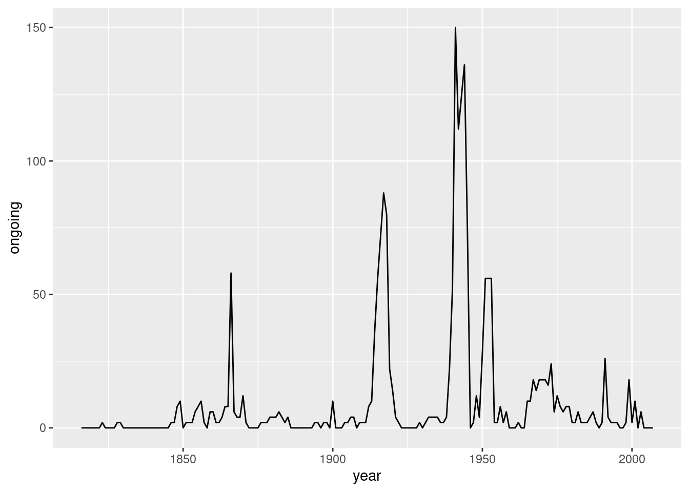
There are many periods, such as the interbellum between the First and Second World Wars, and the “first globalization” from about 1870 to the beginning of the First World War, which were roughly as peaceful, or arguably, more peaceful than present-day.
To take into account the change in the number of countries, we can also plot the percentage of countries that is at war:
stats |>
  ggplot(aes(x = year)) + geom_line(aes(y = ongoing/count))
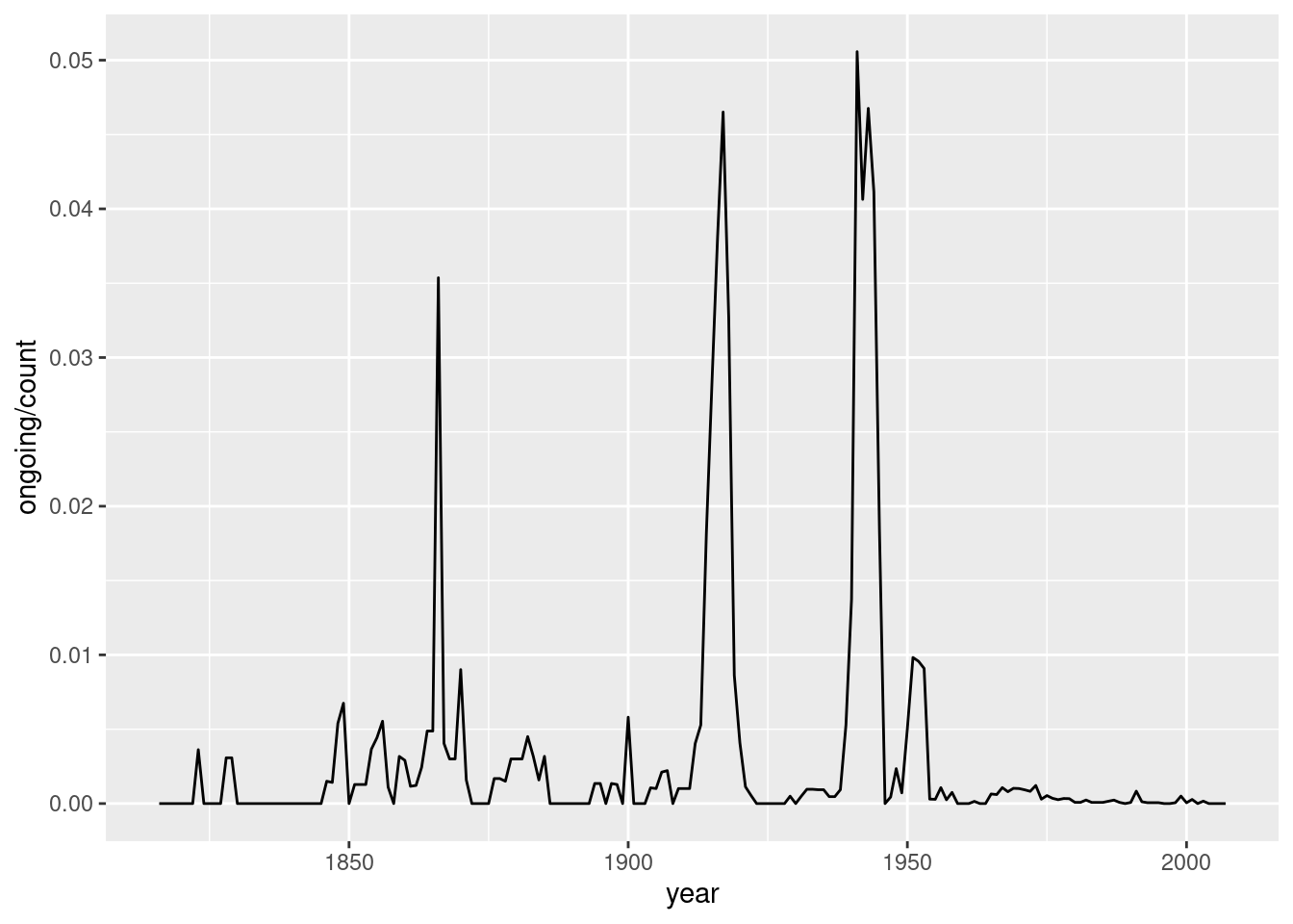
We notice a strong drop in the percentage of countries that go to war from about 1950 onward, reflecting the independence of many countries in the decolonization wave (and the fact that they did not fight among each other).
We can also look at this using some simple models (I estimate linear models, but also Poisson regressions, as the outcome is a count variable):
library(fixest); library(modelsummary)

model1 <- feols(ongoing ~ year, data = stats)
model2 <- feols(started ~ year, data = stats)

model3 <- glm(ongoing ~ year, data = stats, family = poisson(link = "log"))
model4 <- glm(started ~ year, data = stats, family = poisson(link = "log"))

modelsummary(list(model1, model2, model3, model4),
             stars = TRUE)
| (1) | (2) | (3) | (4) | |
|---|---|---|---|---|
| (Intercept) | −127.150* | −42.572 | −12.309*** | −10.926*** |
| (57.165) | (26.134) | (0.848) | (1.322) | |
| year | 0.072* | 0.024+ | 0.008*** | 0.006*** |
| (0.030) | (0.014) | (0.000) | (0.001) | |
| Num.Obs. | 192 | 192 | 192 | 192 |
| R2 | 0.029 | 0.016 | ||
| R2 Adj. | 0.024 | 0.011 | ||
| AIC | 5286.7 | 2419.9 | ||
| BIC | 5293.2 | 2426.5 | ||
| Log.Lik. | −2641.359 | −1207.969 | ||
| F | 299.261 | 87.304 | ||
| RMSE | 22.84 | 10.44 | 23.04 | 10.48 |
| Std.Errors | IID | IID | ||
| + p < 0.1, * p < 0.05, ** p < 0.01, *** p < 0.001 |
These analyses corroborate the conclusions made when eyeballing the graphical pattern above: The time trend is slightly positive, meaning as time goes on, wars are more likely to occur and there is a higher likelihood of a country being involved in a war with another country. However, the time trend is not significant.
However, we might argue that the second World War represents such a shock to humanity that everything is different after 1945. Using only observations after 1945, we see the following pattern:
stats2 <- stats |> filter(year > 1945)

model1 <- feols(ongoing ~ year, data = stats2)
model2 <- feols(started ~ year, data = stats2)

model3 <- glm(ongoing ~ year, data = stats2, family = poisson(link = "log"))
model4 <- glm(started ~ year, data = stats2, family = poisson(link = "log"))

modelsummary(list(model1, model2, model3, model4),
             stars = TRUE)
| (1) | (2) | (3) | (4) | |
|---|---|---|---|---|
| (Intercept) | 519.374** | 117.553 | 65.063*** | 31.897*** |
| (169.558) | (87.508) | (5.218) | (7.368) | |
| year | −0.258** | −0.058 | −0.032*** | −0.015*** |
| (0.086) | (0.044) | (0.003) | (0.004) | |
| Num.Obs. | 62 | 62 | 62 | 62 |
| R2 | 0.131 | 0.027 | ||
| R2 Adj. | 0.117 | 0.011 | ||
| AIC | 868.3 | 566.2 | ||
| BIC | 872.6 | 570.5 | ||
| Log.Lik. | −432.153 | −281.118 | ||
| F | 144.696 | 17.171 | ||
| RMSE | 11.89 | 6.14 | 11.88 | 6.12 |
| Std.Errors | IID | IID | ||
| + p < 0.1, * p < 0.05, ** p < 0.01, *** p < 0.001 |
There is a significant downward time trend in this case, indicating that countries are less likely to wage war with each other since 1945, and that the likelihood of being involved in a war in a given year also decreases.
This could be the result of a lot of factors potentially, among which might be:
- Changes in the international system: the post-WWII order created a sort of hegemonic stability preventing large-scale war between countries.
- Changes in the composition of countries: after the independence of countries from colonialism, many countries were left poor and did not have sufficient resources to devote to belligerence.
- Democratization: many countries became more democratic, and democratic control might prevent countries’ leaders from waging war.
In this blog post, I focus on the last theory and find out whether there is evidence for it. This theory is very frequently encountered in the literature, for example, in Harari’s books, in Steven Pinker’s last book, and in Oded Galor’s last book, though I do not think Galor explicitly endorsed it.
Although all of these books do a good job in anecdotally making their point, and and are much more nuanced than might seem to be the case in this blog post, I think there is a need to tackle this issue from a statistical point of view rather than from a perspective of anecdotes.
Are democratic countries less likely to start wars or be involved in wars?
In order to analyze whether democratic countries are less likely to start a war, we have to obtain data measuring how democratic countries are. Fortunately, the peacesciencer also contains democracy data, featuring three different indicators coming from: the Varieties of Democracy project, the Polity project, and the quickUDS indicators. I’ll focus mainly on the third indicator (quickUDS) because of its broad coverage:
wars_data <- peacesciencer::add_democracy(wars_data)
Now we can analyze the probability of country being in a war as a function of its democracy score. In order to aid interpretability, let us calculate the extent to which the democracy varies from country to country and over time:
wars_data |>
  group_by(ccode1) |>
  summarize(sd = sd(xm_qudsest1, na.rm = T)) |>
  summarize(se = mean(sd), max_se = max(sd), min_se = min(sd))
## # A tibble: 1 × 3
##      se max_se min_se
##   <dbl>  <dbl>  <dbl>
## 1 0.391   1.30      0
This tells us that the average within-country standard deviation is about 0.4, meaning that within countries, on average, the democracy score varies by about 0.4 units on this scale. Some countries have known a much more volatile trajectory, with a standard deviation of about 1.3, whereas other countries have no variation at all.
Another way to shed light on this is just to take a particular case. The Netherlands, for instance, evolved like this:
wars_data |>
  filter(ccode1 == 210) |>
  group_by(year) |>
  summarize(dem_score = mean(xm_qudsest1)) |>
  ggplot(aes(x = year, y = dem_score)) + geom_line()

.. and Albania evolved like this:
wars_data |>
  filter(ccode1 == 339) |>
  group_by(year) |>
  summarize(dem_score = mean(xm_qudsest1)) |>
  ggplot(aes(x = year, y = dem_score)) + geom_line()
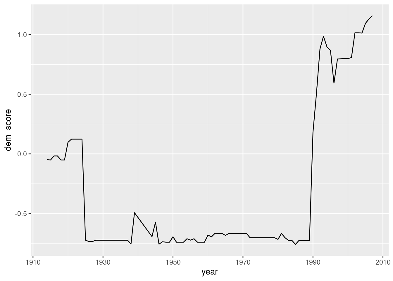
Thus, the switch from communism to a market economy and associated increases in democracy correspond to a jump of about 1.5 on this scale, or about 3 or 4 average intra-country standard deviations, whereas the switch from an absolute monarchy (Netherlands in 1815) to a contemporary liberal democracy (Netherlands in 2007) represents about 2 points.
The average democracy score in the sample is equal to:
wars_data |>
  group_by(ccode1) |>
  summarize(mean = mean(xm_qudsest1, na.rm = T)) |>
  summarize(avg_dem_score = mean(mean))
## # A tibble: 1 × 1
##   avg_dem_score
##           <dbl>
## 1         0.331
Next, we can start to analyze our data. The first thing to do is to restrict our attention to whether country is at, or goes to, war at time with at least 1 other country. I take going to war to mean, to be party in a newly starting war. Hence, this does not distinguish between aggressor and aggressee.
wars_data3 <- wars_data |>
  group_by(ccode1, year) |>
  summarize(xm_qudsest1 = mean(xm_qudsest1, na.rm = T),
            be_in_war = if_else(sum(cowinterongoing, na.rm = T) > 0, 1, 0),
            go_to_war = if_else(sum(cowinteronset, na.rm = T) > 0, 1, 0))
Analyzing this dataset, we discover a very interesting pattern:
model1 <- fixest::feols(go_to_war ~ xm_qudsest1, data = wars_data3)
model2 <- fixest::feols(go_to_war ~ xm_qudsest1 | year, data = wars_data3)
model3 <- fixest::feols(go_to_war ~ xm_qudsest1 | year + ccode1, data = wars_data3)
model4 <- fixest::feols(be_in_war ~ xm_qudsest1, data = wars_data3)
model5 <- fixest::feols(be_in_war ~ xm_qudsest1 | year, data = wars_data3)
model6 <- fixest::feols(be_in_war ~ xm_qudsest1 | year + ccode1, data = wars_data3)

modelsummary(dvnames(list(model1, model2, model3, model4, model5, model6)), stars = T)
| go_to_war | go_to_war | go_to_war | be_in_war | be_in_war | be_in_war | |
|---|---|---|---|---|---|---|
| (Intercept) | 0.028*** | 0.051*** | ||||
| (0.001) | (0.002) | |||||
| xm_qudsest1 | −0.006*** | −0.003 | −0.008** | −0.007** | −0.001 | −0.005 |
| (0.002) | (0.002) | (0.003) | (0.002) | (0.003) | (0.004) | |
| Num.Obs. | 14195 | 14195 | 14195 | 14195 | 14195 | 14195 |
| R2 | 0.001 | 0.087 | 0.121 | 0.001 | 0.107 | 0.178 |
| R2 Adj. | 0.001 | 0.074 | 0.095 | 0.001 | 0.094 | 0.153 |
| R2 Within | 0.000 | 0.001 | 0.000 | 0.000 | ||
| R2 Within Adj. | 0.000 | 0.000 | 0.000 | 0.000 | ||
| RMSE | 0.16 | 0.16 | 0.15 | 0.22 | 0.21 | 0.20 |
| Std.Errors | IID | by: year | by: year | IID | by: year | by: year |
| FE: year | X | X | X | X | ||
| FE: ccode1 | X | X | ||||
| + p < 0.1, * p < 0.05, ** p < 0.01, *** p < 0.001 |
We find that the unconditional relationship between democracy and going to war is negative, consistent with democratic peace theory. The effect is quite small, with a 1 unit increase in the democracy score associated with a 0.8 percentage point decline in the likelihood of being involved in the start of a war.
However, as soon as we condition on a particular year, this relationship disappears for both going to war, and being in a war. I think it is correct to control for year to disentangle possible correlations between times at which wars spiked, like the first World War, or decolonization wars, and concurrent spikes in democracy. Secondly, when we also control for country fixed-effects, the relationship is insignificant in the case for being at war, but significant and negative for going to war, meaning more democratic countries are less likely to be going to war (or to be a party of a starting war), but NOT less likely to be at war. Again, I think controlling for country fixed-effects is correct, because this way, effects like geographical location or regional stability can be disentangled from democracy.
(In contrast, I think that controlling for country times year fixed effects is not correct, because that might reflect things like an increased defense budget, which might be caused by democracies and might change the calculus for going to war or not.)
But, if we condition the data on the period after 1945, we uncover the following pattern:
wars_data4 <- wars_data3 |> filter(year > 1945)

model1 <- fixest::feols(go_to_war ~ xm_qudsest1, data = wars_data4)
model2 <- fixest::feols(go_to_war ~ xm_qudsest1 | year, data = wars_data4)
model3 <- fixest::feols(go_to_war ~ xm_qudsest1 | year + ccode1, data = wars_data4)
model4 <- fixest::feols(be_in_war ~ xm_qudsest1, data = wars_data4)
model5 <- fixest::feols(be_in_war ~ xm_qudsest1 | year, data = wars_data4)
model6 <- fixest::feols(be_in_war ~ xm_qudsest1 | year + ccode1, data = wars_data4)

modelsummary(dvnames(list(model1, model2, model3, model4, model5, model6)), stars = T)
| go_to_war | go_to_war | go_to_war | be_in_war | be_in_war | be_in_war | |
|---|---|---|---|---|---|---|
| (Intercept) | 0.018*** | 0.036*** | ||||
| (0.002) | (0.002) | |||||
| xm_qudsest1 | −0.003+ | −0.001 | −0.002 | −0.005** | −0.001 | 0.003 |
| (0.001) | (0.002) | (0.004) | (0.002) | (0.003) | (0.005) | |
| Num.Obs. | 8766 | 8766 | 8766 | 8766 | 8766 | 8766 |
| R2 | 0.000 | 0.033 | 0.084 | 0.001 | 0.052 | 0.173 |
| R2 Adj. | 0.000 | 0.026 | 0.056 | 0.001 | 0.045 | 0.148 |
| R2 Within | 0.000 | 0.000 | 0.000 | 0.000 | ||
| R2 Within Adj. | 0.000 | 0.000 | 0.000 | 0.000 | ||
| RMSE | 0.13 | 0.13 | 0.12 | 0.18 | 0.17 | 0.16 |
| Std.Errors | IID | by: year | by: year | IID | by: year | by: year |
| FE: year | X | X | X | X | ||
| FE: ccode1 | X | X | ||||
| + p < 0.1, * p < 0.05, ** p < 0.01, *** p < 0.001 |
In this sample, we find that, before controlling for year- and country fixed-effects, there is a negative relationship between democracy and going to / being in a war. This finding might also explain why democratic peace theory is so prevalent. However, after conditioning on country and year fixed effects, the relationship is no longer statistically significant, and its point estimate for being to war is even positive!
Are more democratic less likely to go to war with more democratic countries?
Another thing we can do is more explicitly analyze the dyadic dataset, indicating whether country and are in an armed conflict, as a function of both of their democracy scores. In particular, we estimate the following model:
This deserves some elaboration. When modeling the likelihood of countries and starting/being in a war at time , it makes sense to consider the democracy score of country when modeling the decision of country . As before, we also want to condition on year and country fixed-effects. Our coefficient of interest is , reflecting the likelihood of country going to war with country conditional on country ’s democracy score and fixed effects.
Optionally, we might also add joint country fixed effects to control, for example, for the distance between them.
With , we test whether the likelihood increases/decreases as the democracy score of country changes for a given democracy score of country . This is strictly speaking not an investigation of democratic peace theory, but if more democratic countries are less likely to go to war with more democratic countries (vis-a-vis less democratic countries), this coefficient would be negative.
Also, since dyadic data is symmetric, let us first filter out (without loss of generality) the double observations, and let us also rescale the independent variables to get a more reasonable magnitude of coefficient estimates:
wars_data2 <- wars_data |>
  filter(ccode2 < ccode1) |>
  mutate(xm_qudsest1 = xm_qudsest1 / 10000,
         xm_qudsest2 = xm_qudsest2 / 10000)
Then, we estimate the models:
model1 <- feols(cowinterongoing ~ xm_qudsest1 + xm_qudsest2,
                data = wars_data2)
model2 <- feols(cowinterongoing ~ xm_qudsest1 + xm_qudsest2  | year,
                data = wars_data2)
model3 <- feols(cowinterongoing ~ xm_qudsest1 + xm_qudsest2 | year + ccode1 + ccode2,
                data = wars_data2)
model31 <- feols(cowinterongoing ~ xm_qudsest1 + xm_qudsest2 | year + ccode1 + ccode2 + ccode1*ccode2,
                data = wars_data2)

model4 <- feols(cowinteronset ~ xm_qudsest1 + xm_qudsest2,
                data = wars_data2)
model5 <- feols(cowinteronset ~ xm_qudsest1 + xm_qudsest2 | year,
                data = wars_data2)
model6 <- feols(cowinteronset ~ xm_qudsest1 + xm_qudsest2| year + ccode1 + ccode2,
                data = wars_data2)

model61 <- feols(cowinteronset ~ xm_qudsest1 + xm_qudsest2 | year + ccode1 + ccode2 + ccode1*ccode2,
                data = wars_data2)

modelsummary(dvnames(list(model1, model2, model3, model31,
                          model4, model5, model6, model61)),
             stars = T)
| cowinterongoing | cowinterongoing | cowinterongoing | cowinterongoing | cowinteronset | cowinteronset | cowinteronset | cowinteronset | |
|---|---|---|---|---|---|---|---|---|
| (Intercept) | 0.002*** | 0.001*** | ||||||
| (0.000) | (0.000) | |||||||
| xm_qudsest1 | −2.473*** | −1.144 | −5.192** | −4.844* | −1.381*** | −0.764+ | −2.546* | −2.518* |
| (0.431) | (0.938) | (1.924) | (1.955) | (0.274) | (0.426) | (1.085) | (1.121) | |
| xm_qudsest2 | −5.207*** | −0.768 | −7.884* | −6.069* | −2.542*** | −0.935** | −4.770** | −3.741* |
| (0.427) | (0.554) | (3.296) | (3.054) | (0.271) | (0.339) | (1.816) | (1.712) | |
| Num.Obs. | 786332 | 786332 | 786332 | 786332 | 786332 | 786332 | 786332 | 786332 |
| R2 | 0.000 | 0.021 | 0.030 | 0.074 | 0.000 | 0.011 | 0.014 | 0.029 |
| R2 Adj. | 0.000 | 0.021 | 0.030 | 0.053 | 0.000 | 0.011 | 0.013 | 0.007 |
| R2 Within | 0.000 | 0.000 | 0.000 | 0.000 | 0.000 | 0.000 | ||
| R2 Within Adj. | 0.000 | 0.000 | 0.000 | 0.000 | 0.000 | 0.000 | ||
| RMSE | 0.03 | 0.03 | 0.03 | 0.03 | 0.02 | 0.02 | 0.02 | 0.02 |
| Std.Errors | IID | by: year | by: year | by: year | IID | by: year | by: year | by: year |
| FE: year | X | X | X | X | X | X | ||
| FE: ccode2 | X | X | X | X | ||||
| FE: ccode1 | X | X | X | X | ||||
| FE: ccode1:ccode2 | X | X | ||||||
| + p < 0.1, * p < 0.05, ** p < 0.01, *** p < 0.001 |
This indicates that in the entire dataset, we again have that the more democratic a country, the less likely it is to be involved in a war, even after controlling for another country’s democracy score. Similarly, the more democratic the other country , the less likely there is for country to be involved in a war against it. But again, let us look at the pattern after 1945:
wars_data5 <- wars_data2 |>
  filter(year > 1945)

model1 <- feols(cowinterongoing ~ xm_qudsest1 + xm_qudsest2,
                data = wars_data5)
model2 <- feols(cowinterongoing ~ xm_qudsest1 + xm_qudsest2 | year,
                data = wars_data5)
model3 <- feols(cowinterongoing ~ xm_qudsest1 + xm_qudsest2 | year + ccode1 + ccode2,
                data = wars_data5)
model31 <- feols(cowinterongoing ~ xm_qudsest1 + xm_qudsest2 | year + ccode1 + ccode2 + ccode1*ccode2,
                data = wars_data5)

modelsummary(dvnames(list( model1, model2, model3, model31)), stars  =T,
             title = "Ongoing Wars")
| cowinterongoing | cowinterongoing | cowinterongoing | cowinterongoing | |
|---|---|---|---|---|
| (Intercept) | 0.001*** | |||
| (0.000) | ||||
| xm_qudsest1 | −1.594*** | −1.521* | 2.129+ | 1.685 |
| (0.273) | (0.636) | (1.159) | (1.119) | |
| xm_qudsest2 | −1.623*** | −0.811* | 2.927* | 1.864+ |
| (0.263) | (0.332) | (1.141) | (0.977) | |
| Num.Obs. | 666317 | 666317 | 666317 | 666317 |
| R2 | 0.000 | 0.003 | 0.014 | 0.096 |
| R2 Adj. | 0.000 | 0.003 | 0.013 | 0.072 |
| R2 Within | 0.000 | 0.000 | 0.000 | |
| R2 Within Adj. | 0.000 | 0.000 | 0.000 | |
| RMSE | 0.02 | 0.02 | 0.02 | 0.02 |
| Std.Errors | IID | by: year | by: year | by: year |
| FE: year | X | X | X | |
| FE: ccode2 | X | X | ||
| FE: ccode1 | X | X | ||
| FE: ccode1:ccode2 | X | |||
| + p < 0.1, * p < 0.05, ** p < 0.01, *** p < 0.001 |
model4 <- feols(cowinteronset ~ xm_qudsest1 + xm_qudsest2,
                data = wars_data5)
model5 <- feols(cowinteronset ~ xm_qudsest1 + xm_qudsest2 | year,
                data = wars_data5)
model6 <- feols(cowinteronset ~ xm_qudsest1 + xm_qudsest2 | year + ccode1 + ccode2,
                data = wars_data5)

model61 <- feols(cowinteronset ~ xm_qudsest1 + xm_qudsest2 | year + ccode1 + ccode2 + ccode1*ccode2,
                data = wars_data5)

modelsummary(dvnames(list(model4, model5, model6, model61)), stars = T,
             title = "Start of Wars")
| cowinteronset | cowinteronset | cowinteronset | cowinteronset | |
|---|---|---|---|---|
| (Intercept) | 0.000*** | |||
| (0.000) | ||||
| xm_qudsest1 | −0.587** | −0.620 | 0.072 | −0.206 |
| (0.181) | (0.394) | (0.690) | (0.732) | |
| xm_qudsest2 | −0.571** | −0.371+ | 0.188 | −0.284 |
| (0.174) | (0.211) | (0.771) | (0.762) | |
| Num.Obs. | 666317 | 666317 | 666317 | 666317 |
| R2 | 0.000 | 0.001 | 0.004 | 0.029 |
| R2 Adj. | 0.000 | 0.001 | 0.003 | 0.004 |
| R2 Within | 0.000 | 0.000 | 0.000 | |
| R2 Within Adj. | 0.000 | 0.000 | 0.000 | |
| RMSE | 0.01 | 0.01 | 0.01 | 0.01 |
| Std.Errors | IID | by: year | by: year | by: year |
| FE: year | X | X | X | |
| FE: ccode2 | X | X | ||
| FE: ccode1 | X | X | ||
| FE: ccode1:ccode2 | X | |||
| + p < 0.1, * p < 0.05, ** p < 0.01, *** p < 0.001 |
These two tables show us that, using data after 1945, after controlling for country and country fixed effects, there is no relationship anymore between how democratic a country is and its tendency to engage in war. That means that there is no evidence that as countries become more democratic, they are less inclined to engage (or be engaged) in military conflict with other states. These results hold for both being involved in a war in year , as well as for being involved in the start of a war in year . The last analysis also show that, after controlling for country fixed effects, and cross-country fixed effects, there is no clear relationship for countries to be less likely (or more likely) to be engaged with more democratic countries, conditional on their own democracy.
Conclusion
I do not analyse whether democracy causes peace. That is of course a much more interesting question, but also one which requires better data and, ideally, experimental administering of democraticness, something which is unimaginable. Some researchers have attempted to use the effect of democracies on e.g. economic growth. Perhaps, instruments similar to those could be used to investigate the influence on the likelihood of going to war.
Instead, I only analyze the correlation between democracy and the likelihood of being involved in war. I find that contrary to popular wisdom, the correlation, after controlling for a few simple factors, is essentially zero, and statistically insignificant.
There are a lot of limitations to this analysis. For example, I did not take into account possible dynamic of the sort mentioned before, in that particular democracies might chose autocratic leaders who subsequently go to war. As it is not clear a priori how to tackle these dynamics, I thought it best to leave them.
Finally, in addition to engaging directly in military conflict with other states, there are also various other ways in which less democratic countries could be more belligerent, for example, by financing proxy wars, supporting parties in inter-state conflicts, etc.
- Posted on:
- February 27, 2023
- Length:
- 19 minute read, 3842 words
- See Also: