Inference with Raster Spatial Data in R

May 4, 2023

Introduction

In this blog post, I want to demonstrate how to work with spatial raster data in R. I already have a couple of tutorials on vector data, but in this blog post, I want to focus exclusively on raster data. I’ll be replicating a paper about Roman Roads by Dalgaard et al. (2021), which attempts to identify the persistent influence of Roman roads (built in the Roman empire) on later economic development. The basic identification strategy they use is a controlled approach, where the unit of analysis is a 1x1 longitude times latitude area. They compute the Roman road density for each area that falls within the boundaries of the former Roman empire , defined as the % of surface of the pixel covered by a road. In addition, as outcome variables, they compute the nightlight (and population) density for the same areas and related them to each other, subject to many controls. In this tutorial I’ll only focus on the basic set-up, and conclude with a small (uncontrolled) analysis, and compare the coefficient magnitude to theirs.

Importing the Data

First, I load the necessary libraries:

library(tidyverse)
library(sf)
library(raster)
library(rgdal)
library(terra)

Data Sources

I’ll also be using a variety of data sources. Here, I want to give a short overview of the data sources used in the original paper, and alternative data sources, as well as R packages that make it easy to access these data:

Dependent variables:

Gridded Population of the World
NOAA Nightlights
Alternative Nightlights package
Website with Graphical User Interface
The Oxford Roman Economy Project: Data on Settlements in 500AD
osmdata R package vignette: Data on contemporary roads

Miscellaneous data:

Digital Atlas of the Roman Empire: used to retrieve Oppidum and Roman settlements through an API Interface
Other Roman Empire Datasets

Independent variables:

Major Roman Roads: From the cawd package:
The Oxford Roman Economy Project: Data on Roman Mines
Terrain ruggedness
elevatr R package Vignette: Elevation data through R
Caloric Suitability Index:
Agricultural Suitability: Agricultural Land Use Evaluation System
The climateR package: Package with access to climate data
The climatrends package: Alternative package with access to climate data

Get the roads and the borders

The borders of the Roman Empire around 117AD can be found on this repository. I’ll be using only a small subset of the data to keep down computational and memory load.

links <- 'https://raw.githubusercontent.com/AWMC/geodata/master/Cultural-Data/political_shading/roman_empire_ce_117_extent/roman_empire_ce_117_extent.geojson'
download.file(links, destfile='roman_empire.geojson')

borders <- sf::st_read('./roman_empire.geojson', quiet=T)|> st_as_sf()

# filtered version to make the data computable
borders <- borders |> filter(OBJECTID < 18)
roads <- cawd::darmc.roman.roads.major.sp |> st_as_sf()

numbers <- st_intersects(roads, borders) |> 
  as.data.frame() |> 
  dplyr::select(row.id) |> 
  pull() |> 
  unique()

roads <- roads |> filter(is.element(row_number(), numbers))

ggplot() + geom_sf(data=borders) + 
  geom_sf(data=roads, color='blue')

Import and filter nightlight density

The following has to be run only once to recreate the nightlights data. The nightlights file is from the VNL dataset as linked to above, and saved locally.

# load the raster dataset
raster_data <- raster("./nightlights/VNL_v21_npp_2014_global_vcmslcfg_c202205302300.average_masked.dat.tif")
# Crop the dataset:
raster_data <- crop(x = raster_data, y = borders)
# Or
#raster_data <- crop(x = raster_data, y = extent(borders))

# Limit the max light intensity
raster_data <- raster_data |> clamp(upper = 50)
# Crop the data:
#raster_data <- raster::mask(raster_data, 
#                                 mask = as_Spatial(st_bbox(borders) |> st_as_sfc()))
# Or:
raster_data <- raster::mask(raster_data ,mask=borders)

# Write output
writeRaster(raster_data, "./nightlights/nightlights_re.tif", overwrite=TRUE)

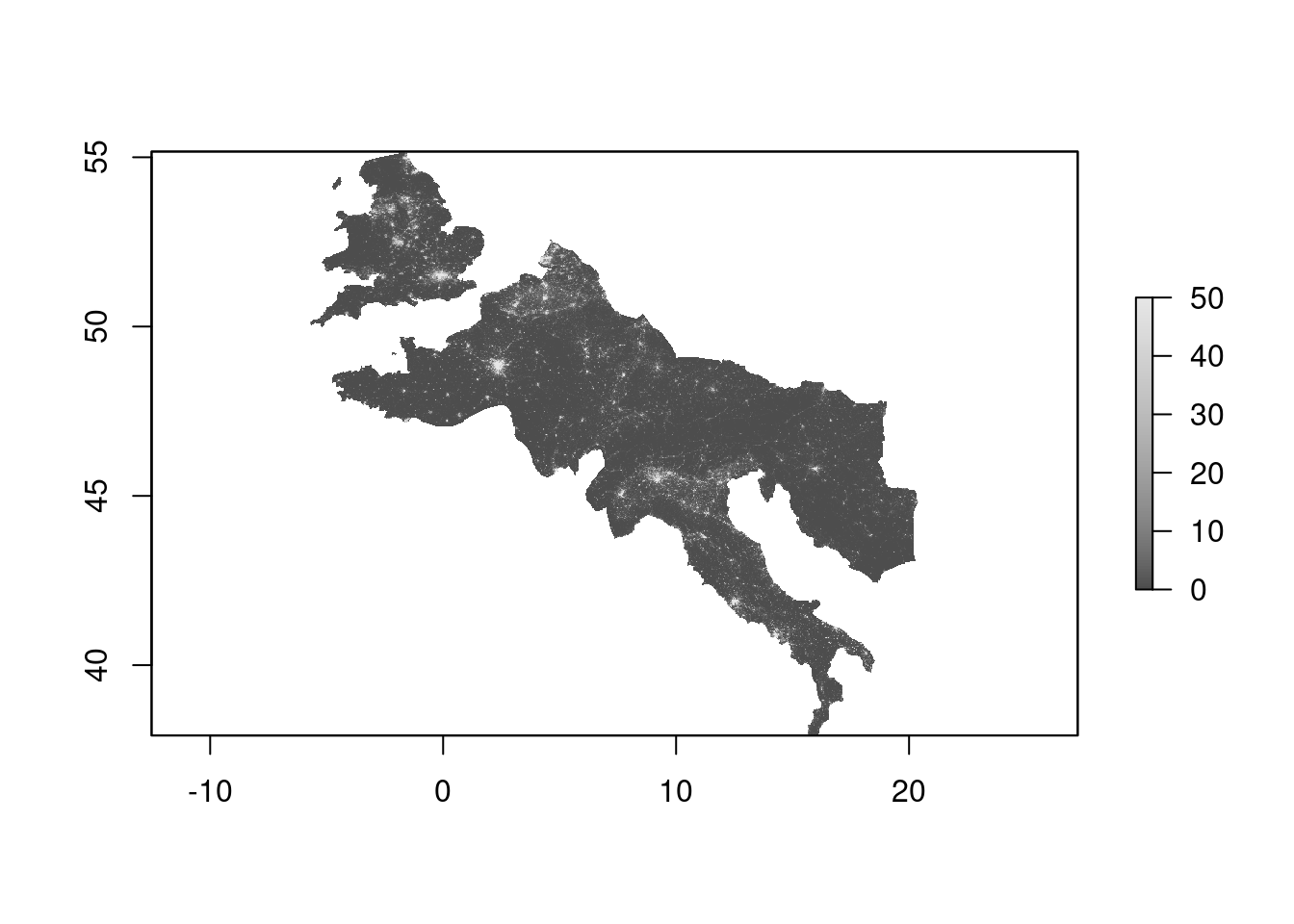
We can now use the imported file:

raster_data <- raster::raster("./nightlights/nightlights_re.tif")
crs <- raster_data@crs

plot(raster_data, col = gray.colors(100))

Compute nightlight density per 0.5x0.5

Now, we can set out to compute the nightlight density per 0.5x0.5 latitude x longitude area.

# set the resolution of the grid
resolution <- 0.5
# convert raster to points
raster_points <- raster::rasterToPoints(raster_data)
# round the coordinates to the nearest 0.5 degrees
raster_points[,1:2] <- round(raster_points[,1:2]/resolution)*resolution
# convert to SpatialPointsDataFrame
raster_sp <- sp::SpatialPointsDataFrame(raster_points[,1:2],
                                        data.frame(value=raster_points[,3]))
# compute mean value for each cell
raster_mean <- raster::aggregate(raster_sp, by=list(round(raster_sp@coords[,1]/resolution),
                                                    round(raster_sp@coords[,2]/resolution)), 
                                 FUN=mean)

# convert back to raster
raster_mean_raster_nl <- raster::rasterFromXYZ(data.frame(raster_mean),
                                            crs=raster_data@crs,
                                            res=resolution)

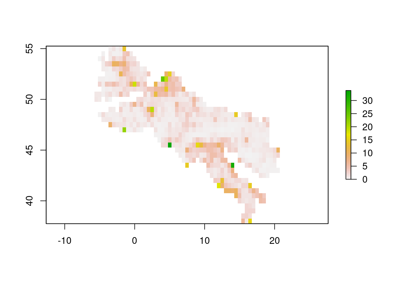
Now our raster looks like this:

plot(raster_mean_raster_nl$value)

Compute Roman Road density per piece of area

Our next job is to calculate the road density over these same areas. In order to do so, we have to create a buffer around the roads to make sure it has an area. In line with the paper, we’ll pick an area of 5 kilometer:

# create a 5km buffer around the vector dataset
buffer_data <- st_buffer(roads, dist = 5000)
# convert the buffer to a raster dataset
buffer_raster <- rasterize(buffer_data, raster_data, background=0)
# reclassify the buffer_raster
buffer_raster <- reclassify(buffer_raster, 
                            matrix(c(0.001, 10000, 1), 
                                   ncol=3, byrow = TRUE)) 

# mask the buffer to be zero only if inside the empire borders but without road
buffer_raster <- mask(buffer_raster, mask = raster_data) 

# convert raster to points
raster_points <- raster::rasterToPoints(buffer_raster)

Now that we have the rasterized buffered roads data, we can aggregate it by 0.5x0.5 latitude x longitude area, and calculate the percentage of area covered by roman road. We reclassified the area such that roads have a value of 1 at a pixel where there is a road, 0 otherwise. Because of this, we can calculate the density by taking the mean per area.

# round the coordinates to the nearest 0.5 degrees
raster_points[,1:2] <- round(raster_points[,1:2]/resolution)*resolution
# convert to SpatialPointsDataFrame
raster_sp <- sp::SpatialPointsDataFrame(raster_points[,1:2],
                                        data.frame(value=raster_points[,3]))

# compute mean value for each cell
raster_mean <- raster::aggregate(raster_sp,
                                 by=list(
                                   round(raster_sp@coords[,1]/resolution),                                                                                     round(raster_sp@coords[,2]/resolution)), 
                                 FUN=mean)

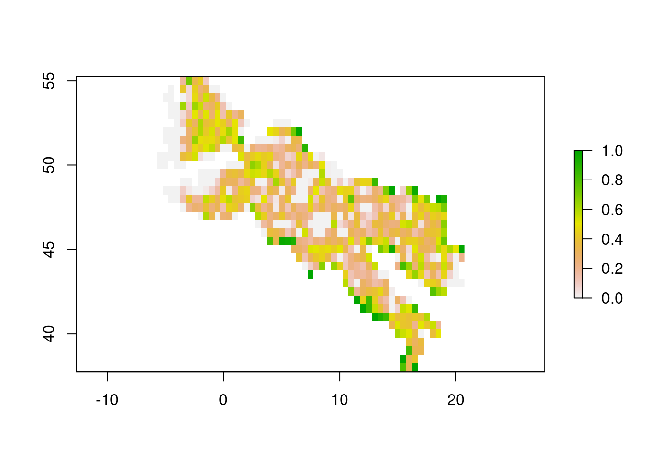
Finally, we put this mean per area back into a raster and plot:

# convert back to raster
raster_mean_raster_roads <- raster::rasterFromXYZ(data.frame(raster_mean),
                                            crs=crs,
                                            res=resolution)

plot(raster_mean_raster_roads$value)

Analysis

The analysis now involves stacking the data from raster_mean_raster_nl (the nightlights data) and raster_mean_raster_roads involving the roads and regression the one on the other. Let’s implement this and then conduct a short analysis. The relevant data is in the fourth column of the raster data. Potentially, we could also merge the data with other data.frames based on the other columns.

data <- data.frame(
  nightlights = raster_mean_raster_nl@data@values[,4],
  roads = raster_mean_raster_roads@data@values[,4])

Now, we estimate the influence of Roman road density on nightlight activity:

library(fixest); library(modelsummary)

fixest::feols(nightlights ~ log(1+roads), data = data) |>
  msummary(stars = T, vcov = 'robust', gof_map = c("adj.r.squared", "nobs"))

	(1)
(Intercept)	1.030***
	(0.239)
log(1 + roads)	5.061***
	(1.062)
R2 Adj.	0.065
Num.Obs.	687
+ p < 0.1, * p < 0.05, p < 0.01, * p < 0.001

The magnitude of the effect is in the same order as that in the paper, although slightly higher. This is likely due to the omission of country fixed effects, which are some of the most important control variables. This is something that could be implemented by iterating through all pieces of area, and asking whether the area is (strictly) inside a particular country. Anyway, I hope this demonstration was useful in explaining how to deal with rastered satellite (and other) data. Thank you for reading.

Posted on:: May 4, 2023

Length:: 6 minute read, 1115 words

See Also: